
Options Essentials & Hedging
1. What you'll learn and why it matters
In Chapter 9 you learned futures: a linear bet where every point the market moves is a point gained or lost. An option is different. It gives one side a choice, and that choice has a price. That changes everything about the payoff, and it makes options the main tool professionals use to insure positions.
This chapter is deliberately narrow. It covers what a swing trader, a long-term investor or a futures trader needs to know about options so they can (a) protect positions, (b) read what the options market is saying about risk, and (c) avoid the traps that cost most retail option traders their money. It does not try to turn you into an options trader.
By the end you will be able to:
- Explain calls and puts, buyers and sellers, and draw all four payoff diagrams with their breakevens.
- Split any premium into intrinsic value and time value, using the real Nifty option chain of 30 Sep 2026.
- Price an option with Black-Scholes, back out its implied volatility, and explain why the model and the market differ.
- Use delta, gamma, theta and vega to predict how a premium will move. We will reconcile a real one-day move to within half a point.
- Read open interest, PCR and max pain, and know how little weight to put on them.
- Build and size a protective put, covered call, collar, bull call spread and bear put spread, with real prices including the March 2026 fall.
- Understand why ~88% of individual F&O traders lost money in FY26 (SEBI), why option buying usually loses, and why option selling can wipe you out in one month.
- Handle expiry, physical settlement of stock options, margins and STT under the rules in force in October 2026.
Swing / positional trader: a put can cap the loss on a position through an event such as results, a budget or an election, which a stop-loss cannot do when the price gaps through it. Long-term investor: a collar or index put can protect a portfolio through a scary period without selling (and triggering capital-gains tax). Futures trader: a long future plus a put has a fixed maximum loss, so a gap cannot take more than you planned. Options also tell you, through implied volatility, how big a move the market expects. That is useful for sizing and stop placement even if you never trade an option.
Options are leveraged, they decay every day, and short options can lose many times the premium collected. SEBI's study of FY26 found that 87.7% of individual equity-derivative traders lost money, and about 92% of those losses came from options. Everything in this chapter is historical analysis for education, not a recommendation to buy or sell any contract.
Don't try to read it in one sitting. Here are three passes:
- Pass 1, the essentials (about 30 min): Sections 2–5 (what an option is, the vocabulary, intrinsic and time value, the four payoffs), then 10.1 (protective put) and 12.1 (what happens at expiry). That is enough to understand a hedge.
- Pass 2, pricing and risk (about 40 min): Section 6 (Black-Scholes, implied volatility), 7 (the Greeks) and 8 (volatility and the expected range). Read these before you pay for any option.
- Pass 3, the rest (about 25 min): Section 9 (option chain), the rest of 10 (covered call, collar, spreads), 11 (why buyers lose and sellers blow up) and 12.2–12.3 (margins and costs).
Sections 6 to 11 each open with a short "In brief" box, so you can come back later and recall the main point quickly.
2. Options in plain language: a right, not an obligation
Suppose you want to buy a flat that costs ₹80 lakh, but you will only know in three months whether you get a job transfer to that city. You pay the builder a non-refundable ₹1 lakh to hold the price at ₹80 lakh for three months. Three things can happen:
- Prices in the area jump to ₹95 lakh. You use your right, buy at ₹80 lakh, and are ₹15 lakh better off before the ₹1 lakh fee, so ₹14 lakh net.
- Prices fall to ₹70 lakh. You walk away. You lose only the ₹1 lakh.
- Prices stay at ₹80 lakh. There is no reason to use the right. You lose the ₹1 lakh.
That fee bought a right without an obligation. The builder took the fee and accepted an obligation: he must sell at ₹80 lakh if you ask. He wins in two of the three scenarios, but his gain is capped at ₹1 lakh while his potential loss is large. That asymmetry between buyer and seller runs through this whole chapter.
| Call option | Put option | |
|---|---|---|
| Buyer (long) pays the premium | Right to buy the underlying at the strike. Profits when price rises. | Right to sell the underlying at the strike. Profits when price falls. This is insurance. |
| Seller / writer (short) receives the premium | Obligation to sell at the strike if exercised. Profits if price stays below the strike. | Obligation to buy at the strike if exercised. Profits if price stays above the strike. |
| Buyer's worst case | Lose the whole premium | Lose the whole premium |
| Seller's worst case | Unlimited (price can keep rising) | Very large (price can fall towards zero) |
The logic. An option splits the upside and downside of an asset and sells one side separately. A put buyer pays to give away the downside below the strike. A call buyer pays to get only the upside above the strike. The premium is the market's price for that slice of risk, so the hard part of options is judging whether the slice is fairly priced. Sections 6 to 8 deal with that.
You rarely have to hold until expiry. A buyer can sell the option back at any time before expiry and book the change in premium. That is how most option positions end.
3. The vocabulary, and how Indian contracts work today
- Underlying: the asset the option is written on, such as the Nifty 50 index or RELIANCE shares.
- Strike price (K): the fixed price at which the buyer may buy (call) or sell (put). NSE lists many strikes. On 30 Sep 2026, the 27-Oct Nifty series had strikes 50 points apart near the money.
- Expiry: the last day the contract lives. After it, the option is settled and disappears.
- Premium: the price of the option, quoted per unit of the underlying. The buyer pays premium × lot size.
- Lot size: the fixed quantity per contract. Nifty is 65 (since the January 2026 series) and RELIANCE is 500. Both figures come from the 30-Sep-2026 bhavcopy.
- Exercise style: all Indian exchange options are European. They are exercised only at expiry, though you can trade out at any time before.
- Settlement: index options are cash-settled at the final settlement price (the index close on expiry day). Stock options that finish in the money are physically settled, meaning shares change hands (Section 12).
- Open interest (OI): the number of contracts still open (Section 9).
Nifty and stock options right now
| Item | Current rule | How verified |
|---|---|---|
| Nifty weekly expiry | Every Tuesday (moved from Thursday on 1 Sep 2025). If Tuesday is a holiday, expiry moves to the previous trading day. | NSE circular / broker notes. The data agrees: the chain shows expiries 06-Oct, 13-Oct and 19-Oct (Monday) because Tue 20-Oct-2026 is the Dussehra holiday. |
| Nifty monthly expiry | Last Tuesday of the month (27-Oct-2026 for October) | Option chain file |
| Stock options expiry | Monthly, last Tuesday (RELIANCE Oct series: 27-Oct-2026) | 30-Sep-2026 bhavcopy |
| Weekly expiries per exchange | One benchmark index per exchange (NSE: Nifty). Bank Nifty has monthly options only. | SEBI circular of 1 Oct 2024, in force since 20 Nov 2024 |
| Nifty lot | 65 units. One lot's notional on 30 Sep 2026 was 22,620.45 × 65 = ₹14,70,329. | Bhavcopy NewBrdLotQty |
4. Moneyness, intrinsic value and time value
4.1 Intrinsic value: what the option is worth if it expired right now
- \(IV_{call},\ IV_{put}\)
- The intrinsic value of a call or a put, in index points (or ₹ per share for a stock option). Here "IV" means intrinsic value. Don't confuse it with implied volatility, also shortened to IV, in Section 6.3.
- \(S\)
- The current spot price of the underlying: the Nifty level or the share price right now.
- \(K\)
- The option's strike price, in the same units as \(S\).
- \(\max(0,\; x)\)
- Means "\(x\) if it is positive, otherwise 0". It picks the larger of 0 and \(x\).
How it works: a call lets you buy at \(K\), so it is worth \(S - K\) if the spot is above the strike. A put lets you sell at \(K\), so it is worth \(K - S\) if the spot is below the strike. If the difference is negative the buyer would simply not exercise, so intrinsic value can never go below 0.
Example (30 Sep 2026, Nifty spot 22,620.45, strike 22600): call \(= \max(0,\; 22{,}620.45 - 22{,}600) = 20.45\) points. Put \(= \max(0,\; 22{,}600 - 22{,}620.45) = \max(0,\; -20.45) = 0\).
4.2 Moneyness
- In the money (ITM): the option has intrinsic value. Calls with \(K < S\), puts with \(K > S\).
- At the money (ATM): the strike closest to spot. On 30 Sep 2026 Nifty closed at 22,620.45, so the ATM strike was 22600.
- Out of the money (OTM): no intrinsic value. Calls with \(K > S\), puts with \(K < S\). Their premium is entirely time value.
The same strike is ITM for one type and OTM for the other. The 23000 strike was an OTM call but an ITM put on 30 Sep 2026.
4.3 Time value: the price of possibility
- Premium
- The option's market price, in points per unit of the underlying. Multiply by the lot size (65 for Nifty) for rupees.
- Intrinsic value
- What the option would be worth if it expired right now (formula above). Zero for an out-of-the-money option.
- Time value
- Everything else in the premium: what buyers pay for the chance that the option gains value before expiry.
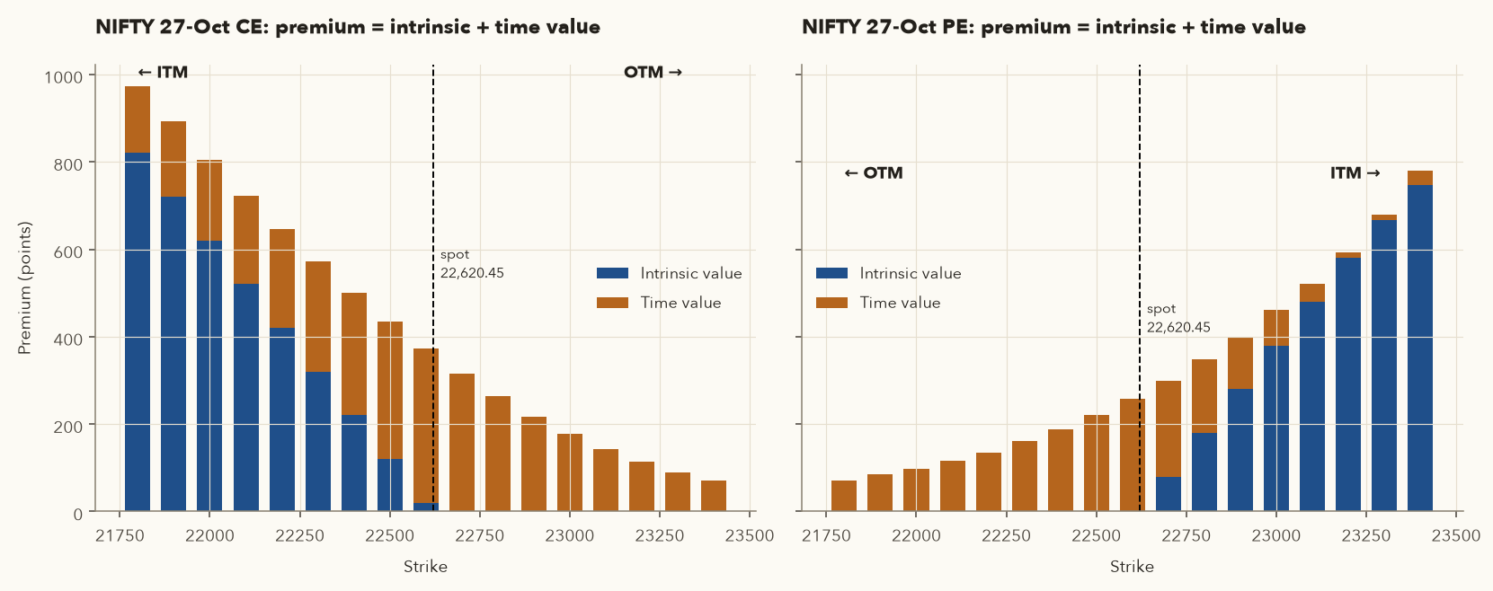
How it works: you can see the premium and work out the intrinsic value, so time value is found by subtraction: time value = premium − intrinsic value. For an OTM option the whole premium is time value. At expiry, time value is zero and the premium equals the intrinsic value.
The logic. Before expiry there is still a chance the option ends up deeper in the money, while the buyer's loss is capped at the premium. The buyer pays for that chance, and the payment is the time value. It is largest at the money, where the outcome is most uncertain, and it shrinks to zero by expiry.
Splitting real premiums (spot 22,620.45, 27 days to expiry)
| Strike | Call | CE premium | Intrinsic | Time value | Put | PE premium | Intrinsic | Time value |
|---|---|---|---|---|---|---|---|---|
| 22000 | ITM | 805.25 | 620.45 | 184.80 | OTM | 98.15 | 0 | 98.15 |
| 22200 | ITM | 646.60 | 420.45 | 226.15 | OTM | 135.50 | 0 | 135.50 |
| 22400 | ITM | 501.15 | 220.45 | 280.70 | OTM | 188.55 | 0 | 188.55 |
| 22600 | ATM | 372.90 | 20.45 | 352.45 | ATM | 258.05 | 0 | 258.05 |
| 22800 | OTM | 264.65 | 0 | 264.65 | ITM | 347.85 | 179.55 | 168.30 |
| 23000 | OTM | 177.80 | 0 | 177.80 | ITM | 460.70 | 379.55 | 81.15 |
| 23200 | OTM | 114.15 | 0 | 114.15 | ITM | 593.25 | 579.55 | 13.70 |
- 22000 CE: intrinsic = max(0, 22,620.45 − 22,000) = 620.45. Time value = 805.25 − 620.45 = 184.80.
- 23000 PE: intrinsic = max(0, 23,000 − 22,620.45) = 379.55. Time value = 460.70 − 379.55 = 81.15.
- Time value peaks near the ATM strike (352.45 for the call, 258.05 for the put) and falls off on both sides.
Why are ATM calls dearer than ATM puts? Interest. Holding Nifty through futures or a call ties up less money than buying the index, so the call carries a "cost of carry". The October future traded at 22,707.30, about 87 points above spot. Put-call parity (Section 6.4) gives an implied forward of 22,715.31. Measured against that forward, the 22600 call is actually slightly ITM and the put slightly OTM.
- Thinking a cheap OTM option is a "bargain". All of its premium is time value, which decays to zero unless the market moves past the strike in time.
- Using stale prices. Illiquid strikes in the bhavcopy can show an old close. For example, the 21050 CE showed 3,282.55 with zero contracts traded that day. Always check volume or the bid-ask spread (the gap between the best price a buyer is offering and the best price a seller is asking) before trusting a premium.
5. The four basic positions and their breakevens
Every option strategy is built from four blocks. Here they are with the real 22600 strike for 27-Oct-2026: call premium 372.90, put premium 258.05. \(S_T\) is the Nifty level at expiry.
- \(S_T\)
- The price of the underlying at expiry (subscript \(T\) = expiry day). For Nifty options this is the final settlement price, the index close on expiry day.
- \(K\)
- The strike price.
- \(C\)
- The call premium paid by the buyer (and received by the seller) at the start, in points per unit.
- \(P\)
- The put premium, in points per unit.
- \(\max(0,\; S_T - K)\)
- What the call is worth at expiry: \(S_T - K\) if Nifty ends above the strike, otherwise 0. For the put it is \(\max(0,\; K - S_T)\).
- Breakeven
- The expiry level at which the position makes exactly zero.
- Work out what the option is worth at expiry using the \(\max(0, \ldots)\) part.
- A buyer (long) gets that value and has already paid the premium, so profit = value − premium. A seller (short) has the mirror image: premium − value.
- The breakeven is where value = premium. A call needs Nifty to finish \(C\) points above the strike, and a put \(P\) points below it. Buyer and seller share the same breakeven.
- The result is in points per unit. Multiply by the lot size (65 for Nifty) and the number of lots to get rupees.
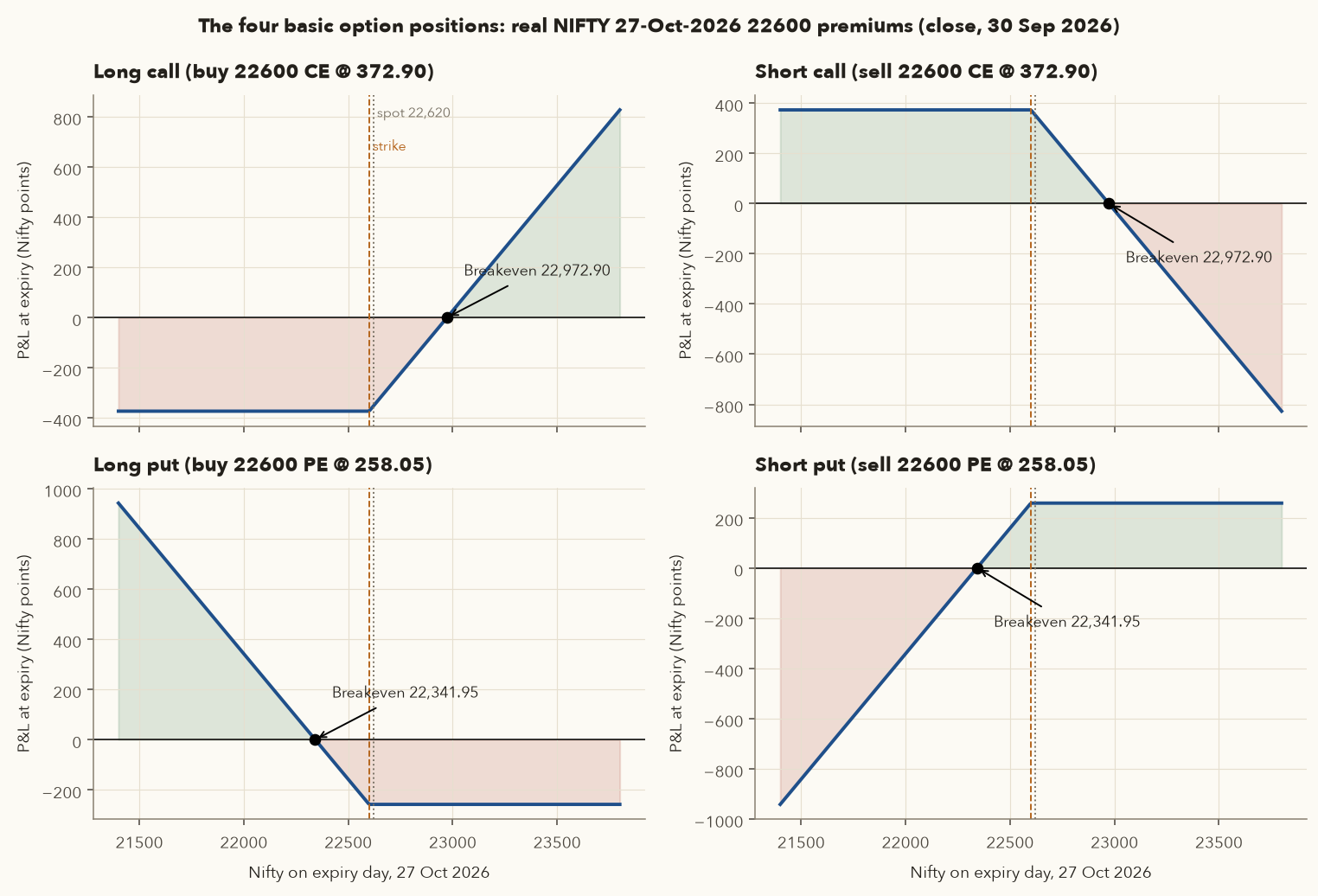
Breakevens and outcomes for one lot (65 units)
- Long call cost: 372.90 × 65 = ₹24,238.50. Breakeven = 22,600 + 372.90 = 22,972.90. Nifty must rise 1.56% from 22,620.45 by expiry just to break even.
- Long put cost: 258.05 × 65 = ₹16,773.25. Breakeven = 22,600 − 258.05 = 22,341.95, a 1.23% fall.
- Outcome table (points per unit at expiry; × 65 for rupees):
| Nifty at expiry | Long call | Short call | Long put | Short put | Long call ₹/lot | Long put ₹/lot |
|---|---|---|---|---|---|---|
| 21,800 | −372.90 | +372.90 | +541.95 | −541.95 | −24,238.50 | +35,226.75 |
| 22,200 | −372.90 | +372.90 | +141.95 | −141.95 | −24,238.50 | +9,226.75 |
| 22,341.95 | −372.90 | +372.90 | 0.00 | 0.00 | −24,238.50 | 0 |
| 22,600 | −372.90 | +372.90 | −258.05 | +258.05 | −24,238.50 | −16,773.25 |
| 22,972.90 | 0.00 | 0.00 | −258.05 | +258.05 | 0 | −16,773.25 |
| 23,400 | +427.10 | −427.10 | −258.05 | +258.05 | +27,761.50 | −16,773.25 |
Note the zone between the breakevens (22,341.95 to 22,972.90). Buyers of either option lose there, and a seller of both (a "short straddle") keeps money there. Most of the time the market ends up in such a zone, which is why option sellers win more often. Section 11 explains why they still get hurt.
5.1 Mapping a view to a position
| Your view | Option ways to express it | Without options | Hedging use |
|---|---|---|---|
| Strongly bullish | Buy call | Buy stock / long futures | Short futures holder buys a call to cap upside risk |
| Mildly bullish / neutral | Sell put, bull call spread | Hold | Covered call on shares you own |
| Strongly bearish | Buy put | Short futures | Protective put on stock or long futures |
| Mildly bearish / neutral | Sell call, bear put spread | Reduce position | Collar |
Profit and loss before expiry (Varsity's M2M chapter) is simpler than it looks. For a buyer it is (exit premium − entry premium) × lot size × number of lots. Buyers pay the full premium upfront, so there is no daily mark-to-market. Sellers post margin, and that margin rises when the premium moves against them (Section 12).
6. What sets the premium: Black-Scholes on a real strike
Five inputs set an option's price: spot, strike, time, interest rate and volatility. Only volatility is unknown, so the price the market pays tells you the volatility it expects (the implied volatility). Black-Scholes is the formula that links them. Use it as a ruler to compare options, not as the "true" value.
6.1 The five inputs, and what each one does
| Input | Effect on call premium | Effect on put premium | Why |
|---|---|---|---|
| Spot price ↑ | ↑ | ↓ | Calls gain intrinsic value, puts lose it |
| Strike ↑ | ↓ | ↑ | The right to buy higher is worth less |
| Time to expiry ↑ | ↑ | ↑ (usually) | More time gives more chance of a big move |
| Volatility ↑ | ↑ | ↑ | Bigger swings make the capped-loss bet more valuable |
| Interest rate ↑ | ↑ (small) | ↓ (small) | Carry: the forward price rises |
Four of these are observable. Volatility is the only input nobody knows, which is why options trading is in large part volatility trading.
6.2 The Black-Scholes formula
- \(C,\ P\)
- The model's fair price for a call and a put, in points per unit.
- \(S\)
- The current spot price (Nifty level or share price).
- \(K\)
- The strike price.
- \(T\)
- Time left to expiry, in years: calendar days ÷ 365. 27 days is 27/365 = 0.074.
- \(r\)
- The risk-free interest rate per year, as a decimal (5.4% = 0.054). A short-term government bill yield is used.
- \(\sigma\)
- The annual volatility of the underlying, as a decimal (13.49% = 0.1349): how much the price typically swings in a year. It is the one input nobody knows for sure.
- \(N(\cdot)\)
- The standard normal cumulative distribution: the area under the bell curve to the left of a number. It turns any number into a probability between 0 and 1. \(N(0) = 0.5\). Excel's
NORM.S.DIST(x, TRUE)gives it. - \(d_1,\ d_2\)
- Two helper numbers that measure how far the spot is above the strike, in units of the expected price swing up to expiry. Near 0 means roughly at the money. The larger they are, the more likely the call is to finish in the money.
- \(\ln,\ e^{-rT},\ \sqrt{\ }\)
- \(\ln\) is the natural logarithm (the
LNkey). \(e^{-rT}\) is a discount factor just below 1, so \(K e^{-rT}\) is the strike's value in today's money. \(\sqrt{\ }\) is the square root.
- Compute \(d_1\) from spot, strike, rate, volatility and time, then \(d_2 = d_1 - \sigma\sqrt{T}\).
- Look up \(N(d_1)\) and \(N(d_2)\). For the put you need \(N(-d_1) = 1 - N(d_1)\) and \(N(-d_2) = 1 - N(d_2)\).
- Call price = spot × \(N(d_1)\) − discounted strike × \(N(d_2)\). The put formula is the mirror image.
- The logic in one sentence: the call is worth the expected value of what you receive at expiry \((S_T)\), counted only when you finish above the strike, minus the discounted strike you pay in those same cases. \(N(d_2)\) is roughly the model's probability of finishing in the money.
Pricing the ATM call by hand
Inputs: \(S\) = 22,620.45, \(K\) = 22,600, \(T\) = 27/365 = 0.07397 years, \(r\) = 5.4% (approximately the 91-day T-bill yield in Sep 2026; the RBI repo rate was 5.25%), \(\sigma\) = India VIX = 13.49%.
- \(\ln(S/K) = \ln(22620.45/22600) = 0.00090\)
- \((r + \sigma^2/2)T = (0.054 + 0.1349^2/2) \times 0.07397 = 0.00467\)
- \(\sigma\sqrt{T} = 0.1349 \times 0.27198 = 0.03669\)
- \(d_1 = (0.00090 + 0.00467)/0.03669 = 0.1519\), and \(d_2 = 0.1519 - 0.0367 = 0.1152\)
- \(N(d_1) = 0.5604\), \(N(d_2) = 0.5458\), and \(K e^{-rT} = 22{,}509.90\)
- \(C = 22620.45 \times 0.5604 - 22509.90 \times 0.5458 = 12{,}675.48 - 12{,}286.99 \approx \mathbf{388.48}\)
- The market price was 372.90, 15.58 points below the model. The same model gives the 22600 PE at 277.94 against a market price of 258.05.
6.3 Model vs market, and implied volatility
Run the formula backwards: find the \(\sigma\) that makes the model price equal the market price. That number is the implied volatility (IV), the volatility the market is charging for. For the 22600 CE at 372.90 it comes out at 12.85%, below India VIX at 13.49%.
| Strike | Type | Market | B-S @ VIX 13.49% | Market − model | Implied vol |
|---|---|---|---|---|---|
| 22000 | PE | 98.15 | 87.13 | +11.02 | 14.14% |
| 22200 | PE | 135.50 | 133.89 | +1.61 | 13.57% |
| 22400 | PE | 188.55 | 196.89 | −8.34 | 13.12% |
| 22600 | CE | 372.90 | 388.48 | −15.58 | 12.85% |
| 22600 | PE | 258.05 | 277.94 | −19.89 | 12.67% |
| 22800 | CE | 264.65 | 289.28 | −24.63 | 12.48% |
| 23000 | CE | 177.80 | 208.85 | −31.05 | 12.15% |
| 23200 | CE | 114.15 | 145.98 | −31.83 | 11.94% |
Why the gaps? (1) India VIX blends many strikes across the two nearest monthly expiries, so it is not the IV of any single option. (2) The market charges more for downside puts (22000 PE at 14.14% IV) than for upside calls (23200 CE at 11.94%). Black-Scholes assumes one volatility for every strike, so it misprices both wings (Section 8.4). (3) Closing prices are snapshots, and the model ignores dividends. Treat Black-Scholes as a consistent ruler for comparing options, not as the true value. Varsity's Greek-calculator chapter uses it the same way: when the market price is well above the model at a sensible volatility, the option is expensive relative to that volatility.
6.4 Put-call parity: why calls and puts are tied together
- \(C,\ P\)
- Market premiums of a call and a put with the same strike and the same expiry, in points.
- \(S\)
- The current spot price.
- \(K e^{-rT}\)
- The strike \(K\) discounted to today's money at interest rate \(r\) for \(T\) years (as in Black-Scholes above). For the 22600 strike with 27 days left it is 22,509.90.
- Long forward at \(K\)
- An agreement to buy the underlying at price \(K\) on the expiry date, similar to a futures contract.
How it works: buying the call and selling the put at the same strike means you end up owning the underlying at \(K\) on expiry whichever way the market goes. That combination must cost the same as owning it via a forward, so call minus put must equal spot minus the discounted strike. If the two sides drift apart, traders buy the cheap side and sell the dear side until the gap closes.
Check with real numbers: \(C - P = 372.90 - 258.05 = 114.85\). The right side is \(22{,}620.45 - 22{,}509.90 = 110.55\). They differ by about 4 points (under 0.02% of spot). That is small enough to come from closing prices struck at slightly different moments and from our 5.4% interest-rate assumption. (Expected dividends would push the gap the other way, so they are not the explanation.) Rearranged, the implied forward is \(K + (C-P)e^{rT} = 22{,}715.31\), close to the actual October future at 22,707.30. If the gap were large, traders would buy the cheap side and sell the dear side until it closed. Varsity's "synthetic long & arbitrage" chapter covers this. One practical point follows: long futures + long put behaves like a long call, which is exactly what a protective put is.
7. The Greeks: delta, gamma, theta, vega
Delta: points gained per point the index moves. Gamma: how fast delta changes, which becomes extreme near expiry. Theta: what you lose each day if nothing happens, and the loss speeds up near expiry. Vega: points gained per 1-point rise in implied volatility. A premium moves on all four at once. In our real one-day example, delta explained only half the move.
The Greeks measure how the premium responds when one input changes and the others are held still. Here are the Black-Scholes Greeks for our two ATM options (27-Oct, vol 13.49%):
7.1 Delta: how much the premium moves per point of the underlying
- \(\Delta\)
- Delta: points the option premium changes for a 1-point move in the underlying.
- \(V\)
- The option's value (its premium), in points.
- \(S\)
- The spot price of the underlying.
- \(\frac{\partial V}{\partial S}\)
- Calculus shorthand for "the change in \(V\) for a small change in \(S\), with everything else (time, volatility, rate) held still".
- \(N(d_1)\)
- The same Black-Scholes quantity as in Section 6.2.
- \(\in [0,1]\)
- "Lies between 0 and 1". A call's delta is between 0 and 1. A put's is between −1 and 0.
How it works: multiply delta by the index move to estimate the premium change. A call delta of 0.56 and a 100-point rise gives about +56 points. A put delta of −0.44 and a 100-point rise gives about −44 points. The estimate holds only for small moves, because delta itself changes as the spot moves (gamma, Section 7.2).
- Meaning: a delta of 0.56 means that if Nifty rises 100 points, the call gains about 56 points, other things equal. A put delta of −0.44 means the put gains about 44 points when Nifty falls 100.
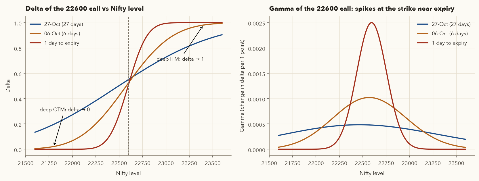
- By moneyness: deep ITM is close to 1 (behaves like the underlying), ATM is about 0.5, deep OTM is close to 0. As expiry approaches, delta moves towards 0 or 1 more sharply (Figure 3).
- As a rough probability: traders read delta as the chance of finishing ITM. The cleaner model number is \(N(d_2)\) = 0.546 for the 22600 call, close to its delta of 0.560.
- Deltas add. A position's delta is the sum of its legs. Long one future (delta +1) plus a long 22600 PE (−0.44) gives net +0.56 per unit, the same as a call. Roughly two ATM calls (2 × 0.56 ≈ 1.1) carry the directional exposure of one future. This is how you measure how much directional exposure a hedge has left.
7.2 Gamma: how fast delta changes
Gamma is delta's rate of change, the "acceleration" to delta's "speed". With gamma 0.00048, a 100-point rise lifts the call's delta from about 0.56 to about 0.61. Gamma is highest at the money and, crucially, it explodes at the money as expiry approaches (right panel of Figure 3). On the last day, an ATM option can swing from nearly worthless to worth a lot within a few dozen index points. That is a gift to the buyer and a danger to the seller. Varsity's rule follows from it: avoid being short ATM options close to expiry.
7.3 Theta: time decay
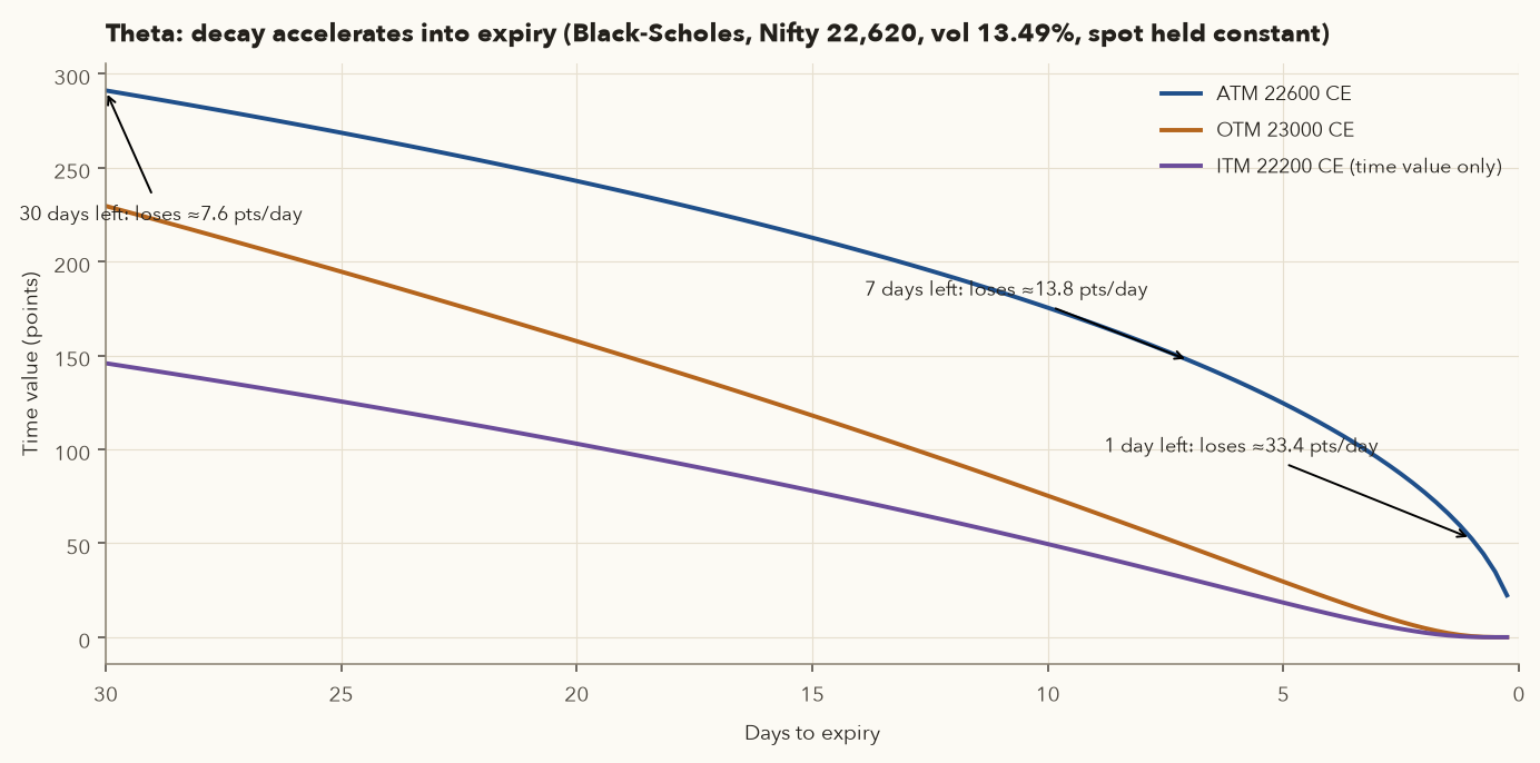
Theta is how much premium is lost per day with everything else unchanged. Buyers have negative theta and sellers have positive theta. Decay is not linear: with spot held at 22,620 and vol at 13.49%, the ATM call's Black-Scholes theta is about −7.6 points a day with 30 days left, −13.8 with 7 days left and −33.4 with one day left. Even that understates the last day, because theta keeps speeding up through it: the ATM call still has about 56 points of time value with one day to go, and all 56 are gone by the close on expiry day.
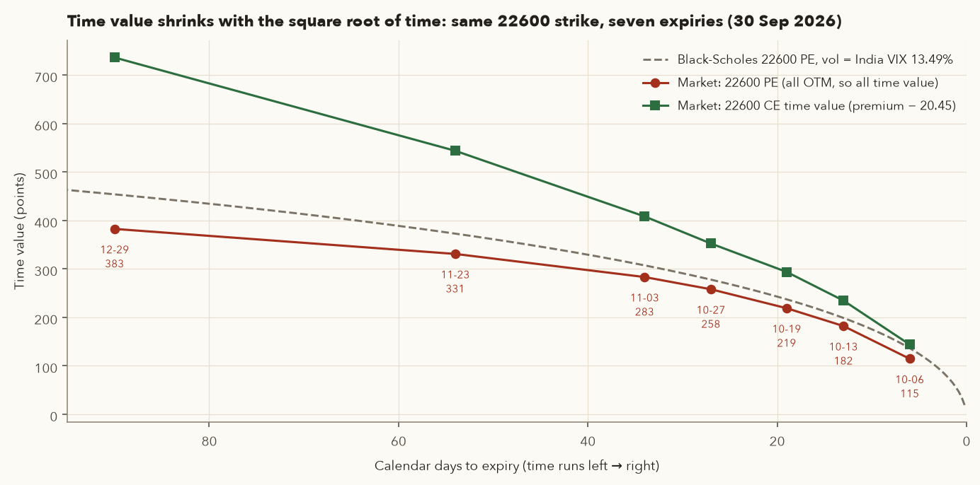
Time value really does scale with √time
The chain gives us something better than a model: the same strike across seven expiries on the same day.
| Expiry | Days | 22600 PE (all time value) | 22600 CE | CE time value |
|---|---|---|---|---|
| 06-Oct-2026 | 6 | 114.65 | 164.50 | 144.05 |
| 13-Oct-2026 | 13 | 182.20 | 255.20 | 234.75 |
| 19-Oct-2026 | 19 | 218.95 | 314.25 | 293.80 |
| 27-Oct-2026 | 27 | 258.05 | 372.90 | 352.45 |
| 03-Nov-2026 | 34 | 283.25 | 428.75 | 408.30 |
| 23-Nov-2026 | 54 | 330.95 | 564.15 | 543.70 |
| 29-Dec-2026 | 90 | 382.55 | 756.65 | 736.20 |
The 90-day put costs 382.55, only about 3.3× the 6-day put (114.65), even though it lasts 15× as long. √(90/6) ≈ 3.9, so the shape is roughly square-root. For a hedger this is a big deal: insurance per day is far cheaper on longer-dated options. Rolling weekly puts is the most expensive way to hedge. The call's time value grows faster than the put's because of carry (the forward rises with time). The 03-Nov and 29-Dec contracts traded very thinly (43 and 29 call contracts), so treat those prices as indicative.
7.4 Vega: sensitivity to volatility
Vega is the change in premium for a 1-percentage-point change in implied volatility. It is the same for a call and a put at the same strike, and both gain when volatility rises. The 22600 options have vega ≈ 24.26, so a rise in IV from 13% to 15% adds about 48 points to both the call and the put, even if Nifty does not move. Vega is larger for longer-dated options and shrinks towards expiry. For hedgers this means: buy protection when IV is calm, not in the middle of a panic. On 27 Feb 2026 India VIX was 13.70. By 30 Mar 2026 it was 27.89 and every put was far more expensive.
Reconciling a real one-day premium change with the Greeks
On 30 Sep Nifty fell from 22,716.20 to 22,620.45 (ΔS = −95.75). Using each option's Greeks as of 29 Sep (computed at its own implied vol), we can explain the move term by term:
- \(\Delta V\)
- The change in the option premium over the day, in points. Here a \(\Delta\) placed in front of a symbol means "change in".
- \(\Delta\) (alone)
- The option's delta, from the previous day.
- \(\Delta S\)
- The change in Nifty over the day, in points (−95.75 here).
- \(\Gamma\)
- Gamma: how much delta changes per 1-point move. \((\Delta S)^2\) is the index move squared, so this term is always positive for a buyer.
- \(\Theta\)
- Theta: points the premium loses per day if nothing else changes. Negative for a buyer.
- Vega
- Points the premium changes for a 1-percentage-point change in implied volatility.
- \(\Delta\sigma\)
- The change in the option's implied volatility over the day, in percentage points (14.76% → 12.85% is −1.91).
- \(\approx\)
- "Approximately equal": the Greeks give an estimate, not an exact answer.
How it works: each term is one cause of the price change: direction (delta), the bend in delta (gamma), one day of time decay (theta) and the change in volatility (vega). Work out the four pieces, add them, and compare with the actual change. The table below does this line by line.
| Term | 22600 CE | 22600 PE |
|---|---|---|
| Delta × ΔS | 0.5976 × −95.75 = −57.22 | −0.3834 × −95.75 = +36.71 |
| ½ Gamma × ΔS² | +1.91 | +2.33 |
| Theta (1 day) | −8.35 | −3.81 |
| Vega × ΔIV | 24.35 × (12.85 − 14.76) = −46.56 | 24.02 × (12.67 − 11.95) = +17.31 |
| Predicted change | −110.23 | +52.54 |
| Actual change (483.00 → 372.90 / 205.35 → 258.05) | −110.10 | +52.70 |
Lesson: delta alone predicted −57 for the call, about half the real loss. The other half came from a fall in the call's implied vol. A trader who bought that call "because delta is 0.6" would have been surprised. Premiums move on direction, time and volatility together. (The exact split depends on closing-price snapshots; the call's and put's IVs moved in opposite directions here partly for that reason.)
7.5 How the Greeks interact (Varsity's rules of thumb)
- Early in the series, gamma is low everywhere and theta is gentle. There is time for a view to play out, and ATM or slightly OTM strikes are reasonable for a buyer.
- Late in the series, ATM gamma and theta both spike. Buyers need the move quickly, and sellers face sudden delta jumps.
- When volatility is high, deep OTM options keep a meaningful delta. When it is low, they behave like lottery tickets.
- Strike choice for a directional buyer should depend on how soon you expect the move. If the move should come within a few days, OTM strikes give the most leverage. If it may take until expiry, ITM strikes are better because their intrinsic value cushions decay. A far-OTM buy that needs a large move and has plenty of time to wait is usually the worst combination.
8. Volatility: historical, implied, India VIX and the skew
Historical volatility measures how much Nifty did move. India VIX measures how much option prices say it will move. VIX has usually been higher than the move that followed, which is why insurance costs a little more than it pays out on average. Spot × VIX × √(days/365) gives the market's 1-standard-deviation range, which you can use for stops and hedge strikes even if you never trade an option.
8.1 Historical volatility: the calculation
- \(P_t,\ P_{t-1}\)
- The closing price on day \(t\) and on the trading day before it.
- \(r_t\)
- The daily log return for day \(t\). \(\ln\) is the natural logarithm. For small moves it is almost the same as the ordinary % change (a 1% rise gives \(r_t \approx 0.00995\)).
- stdev
- The standard deviation: a measure of how widely the daily returns spread around their average (Chapter 11 works one out by hand).
- \(\sigma_{daily}\)
- Historical volatility per trading day.
- 252
- The approximate number of trading days in a year.
- \(\sigma_{annual}\)
- The same volatility scaled up to one year, the form option prices and India VIX use.
- \(N\), \(\sigma_{N\text{-day}}\)
- A number of trading days, and the volatility over that many days.
- Turn each pair of closes into a log return. A year of data gives about 252 returns.
- Take the standard deviation of those returns. That is the daily volatility.
- Multiply by \(\sqrt{252}\) to annualise, or by \(\sqrt{N}\) for an \(N\)-day period. Volatility grows with the square root of time, not in a straight line, because up days and down days partly cancel.
From daily returns to annual volatility
- Take the last 252 daily log returns of Nifty up to 30 Sep 2026. Their standard deviation is 0.8347% per day.
- Annualise: 0.8347% × √252 = 13.25%.
- The last 20 days alone gave only 10.19%, because September was a steady grind lower rather than a series of big daily swings.
- India VIX on 30 Sep 2026: 13.49%. The options market expected the next 30 days to be roughly as volatile as the past year and more volatile than the past month.
8.2 Implied volatility and India VIX
Historical vol looks back. Implied vol is the forward-looking number embedded in option prices. India VIX is NSE's index of the 30-day implied volatility of Nifty, computed from the order book of near and next-month Nifty options. It is often called the "fear index" because it jumps when markets fall.
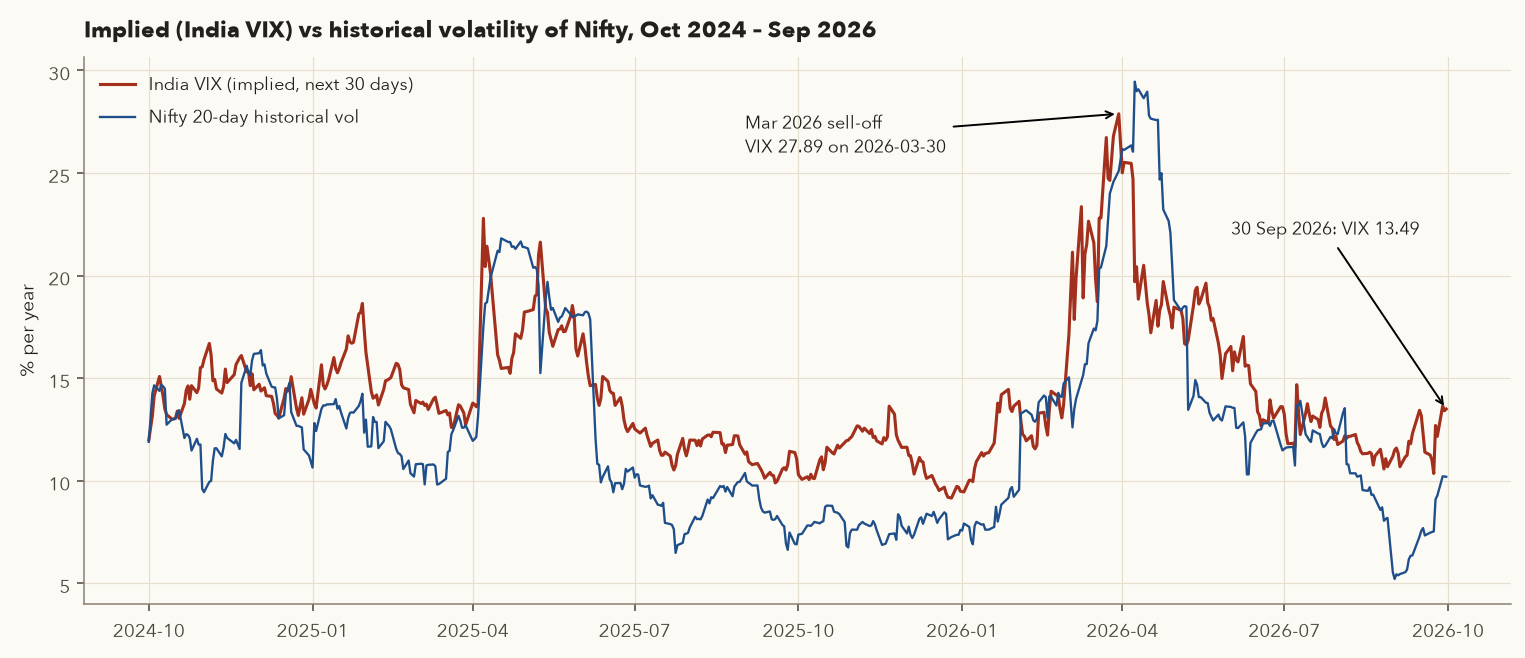
From 2016 to Sep 2026, India VIX was higher than the volatility Nifty actually delivered over the following 20 trading days on 81.1% of days, by 2.62 vol points on average. Option buyers, as a group, pay a little more than fair for insurance, much as house insurance costs more than the average claim. That is the structural reason option buying loses on average. The other 19% of the time, realised volatility overshoots and the seller pays out heavily. Section 11 shows both sides.
8.3 Using volatility to estimate an expected range
- 1 SD move
- One standard deviation move, in index points: the size of move the market prices as "normal" over the period.
- \(S\)
- The current spot level.
- \(\sigma_{annual}\)
- Annual volatility as a decimal. Usually India VIX ÷ 100 (13.49 → 0.1349), or an option's implied volatility.
- \(N\)
- The number of calendar days until the date you care about (for example expiry).
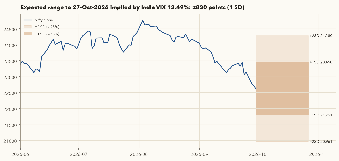
How it works: \(\sqrt{N/365}\) shrinks the yearly volatility down to the period you care about. Multiplying by spot turns that percentage into points. Spot ± 1 SD is the range the market expects Nifty to stay inside about 68% of the time (if returns were normal), and spot ± 2 SD about 95% of the time.
Which day count? India VIX and option-pricing time \(T\) are quoted on a calendar-day basis, so with VIX you scale by \(\sqrt{N/365}\) where \(N\) is calendar days. Historical volatility in 8.1 was built from trading-day returns, so it scales by \(\sqrt{252}\) and \(\sqrt{N_{trading}}\). Both give about the same answer for the same period. Mixing them, for example VIX with \(\sqrt{N/252}\) on calendar days, overstates the range.
What range is the market pricing?
- 27 calendar days: 13.49% × √(27/365) = 3.67%.
- 1 SD = 22,620.45 × 3.67% ≈ 830 points, so the ±1 SD range is 21,791 to 23,450 (roughly 68% probability if returns were normal).
- ±2 SD is 20,961 to 24,280 (roughly 95%).
- Cross-check from prices alone: the ATM straddle (22600 CE + PE) cost 372.90 + 258.05 = 630.95, or 2.79% of spot. A straddle's price is roughly 0.8 × the 1-SD move (630.95 / 0.8 ≈ 790), so the two estimates agree reasonably. The 06-Oct weekly straddle cost 279.15, against a 1-SD move of about 391 points for 6 days.
Uses. A swing trader can compare a planned stop with this range: a stop well inside one day's or one week's normal noise will be hit by randomness. A hedger can see which put strikes the market thinks are unlikely, and therefore cheap. Varsity uses the same range to pick strikes for option writing. Remember, though, that real returns have fatter tails than the normal curve: moves beyond 2 SD happen far more often than 5% of the time.
8.4 The volatility skew (smile)
If Black-Scholes were exactly right, every strike would have the same IV. In reality, Nifty puts below spot carry higher IV than calls above it. On 30 Sep 2026 the 27-Oct 21600 PE traded at 15.44% IV, while the 23400 CE traded at 11.87%. The logic: markets fall faster than they rise, and institutions buy downside puts as insurance, so crash protection carries a premium. The weekly expiry shows a true "smile" (both wings up, from 11.59% at 22600 to 17.86% at 21600 and 15.95% at 23600) because very short options price jump risk on both sides.
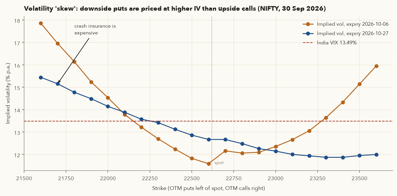
Practical consequence: far-OTM puts cost more than a flat-volatility model suggests, so the "cheapest" hedge in rupees is not the cheapest in volatility terms. Selling an OTM call against a put (a collar, Section 10.3) partly pays for this expensive downside protection with cheaper upside.
9. Reading the option chain: OI, PCR and max pain
The option chain shows where open positions sit. Open interest, the put-call ratio and max pain describe that positioning, but they do not predict where Nifty will go. Use them as background only.
An option chain lists every strike for one expiry, with calls on the left and puts on the right: last price, change, volume, open interest (OI) and change in OI. On NSE's chain and broker apps, ITM strikes are shaded.
9.1 Open interest by strike
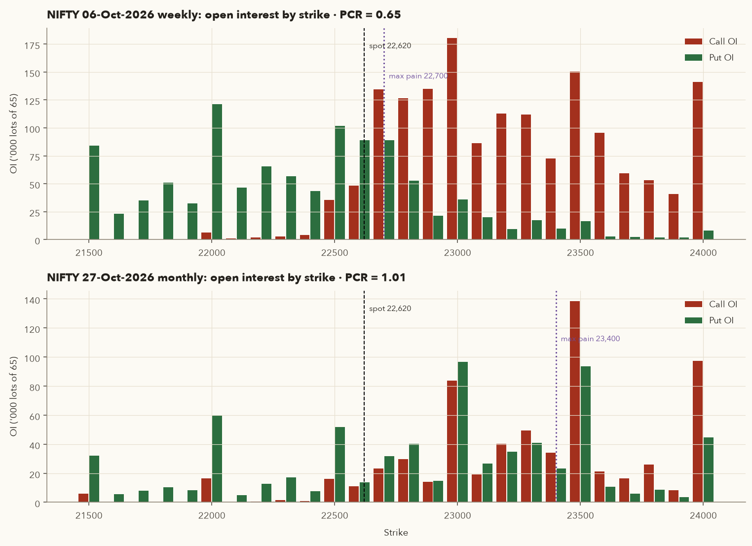
OI counts contracts open at the end of the day. Every contract has a buyer and a seller, so OI does not tell you who is "right". The common reading is that heavy call OI at a strike above spot is where call writers expect a ceiling, and heavy put OI below spot is where put writers expect a floor. It reflects positioning, not a guarantee.
9.2 Put-call ratio (PCR)
- \(PCR\)
- The put-call ratio: a plain number with no units.
- Total put OI
- The open interest of every put, added across all strikes of the expiry (or expiries) you choose.
- Total call OI
- The same total for calls, over the same expiries.
How it works: add up open interest for puts and for calls, then divide. Above 1 means more puts are open than calls, below 1 the reverse. Lots or units give the same ratio, as long as you use the same measure for both. The answer changes a lot depending on which expiries you include, as the table shows.
PCR depends heavily on which expiry you look at
| Scope | Put OI (lots) | Call OI (lots) | PCR |
|---|---|---|---|
| 06-Oct weekly | 1,629,584 | 2,524,177 | 0.646 |
| 27-Oct monthly | 947,048 | 936,040 | 1.012 |
| All expiries | — | — | 0.788 |
Interpretation. Varsity treats PCR as a contrarian gauge. A very high PCR (it cites about 1.3 or more) means extreme pessimism and possibly a bounce. A very low one (about 0.5 or less) means complacency. Our readings are in the "normal" band, and the weekly and monthly figures disagree, which is typical. Use PCR as background, and only with your own back-test of its thresholds on Nifty.
9.3 Max pain
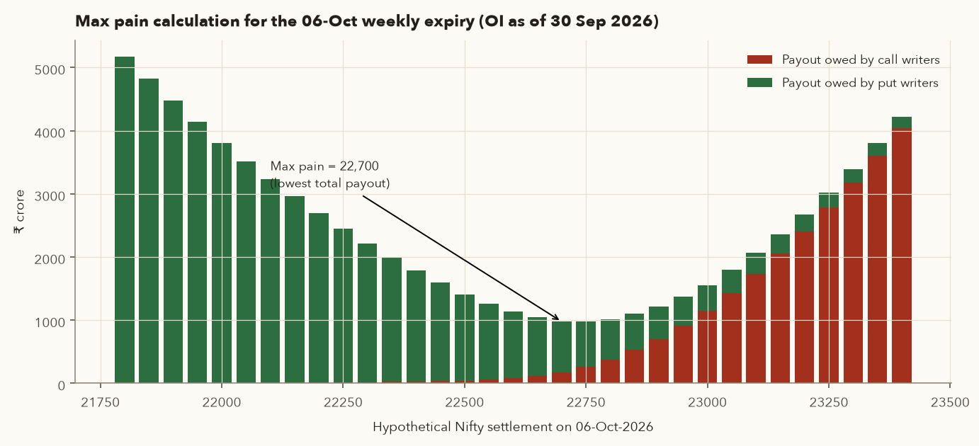
Idea: at expiry, option writers as a group pay out the least if the index settles at one particular strike. "Max pain" theory says the market tends to drift towards that level into expiry.
- \(X\)
- A possible settlement level for the index at expiry. Each listed strike is tried in turn.
- \(K\)
- A strike in the option chain.
- \(OI^{call}_K,\ OI^{put}_K\)
- Open interest of the call and of the put at strike \(K\), counted in units (lots × 65), so the pain comes out in rupees.
- \(\max(0,\; X-K)\)
- What one unit of the \(K\) call is worth if Nifty settles at \(X\): \(X - K\) if positive, otherwise 0 (Section 4.1). \(\max(0,\; K-X)\) is the same for the put.
- \(\sum_K\)
- "Add this up over every strike \(K\)."
- \(\text{Pain}(X)\)
- The total ₹ that option writers would have to pay buyers if the index settled at \(X\).
- \(\arg\min_X\)
- "The value of \(X\) that makes the expression smallest." It returns the level, not the amount.
- Pick a settlement level \(X\).
- For every strike, multiply open interest by what that option would be worth at \(X\). Add up all calls and all puts.
- Repeat for every candidate \(X\). The level with the smallest total is the max-pain level.
Computing max pain step by step
- For each candidate settlement X, add up what every call writer would owe (call OI × max(0, X − K)) and every put writer would owe (put OI × max(0, K − X)). OI is in units, so the result is in rupees.
- Selected results (₹ crore):
| Settlement X | Call writers owe | Put writers owe | Total |
|---|---|---|---|
| 22,400 | 27.46 | 1,764.54 | 1,792.00 |
| 22,600 | 81.21 | 1,051.47 | 1,132.68 |
| 22,700 | 168.11 | 809.15 | 977.25 (minimum) |
| 22,800 | 374.89 | 640.72 | 1,015.60 |
| 23,000 | 1,144.90 | 409.45 | 1,554.35 |
Weekly max pain = 22,700, close to spot. The monthly max pain was 23,400, almost 800 points above spot, because much of that OI was built in early September with Nifty near 24,000. That is a good example of why max pain is unreliable on its own. It is computed from yesterday's positions, it shifts daily, and it has little academic support. Varsity's author suggests looking at it about 15 days before expiry with a buffer, as context for writing far-OTM options, not as a target.
- OI is a snapshot, while positions are opened and closed all day.
- Many "writers" are hedged (for example, a fund long stock and short calls), so their OI says nothing about direction.
- Large OI at a strike can attract volatility rather than stop it.
- Use the chain for context (expected range, where protection is cheap or expensive), never as a stand-alone signal.
10. Hedging with options: five structures with real prices
A protective put sets a hard floor for a premium. A collar pays for that floor by giving up gains above a cap. A bear put spread is cheap protection against a moderate fall only. A covered call earns a little income and is not a hedge. For a stock portfolio, size index puts by beta, and plan for physical settlement on stock options.
A hedge is something you hold alongside a position so that a bad outcome hurts less. It always costs something: cash (a premium), upside (a cap) or both. The question is never "is there a free hedge?" but "which cost am I willing to pay?"
10.1 Protective put: insurance with a fixed deductible
- \(S_0\)
- The price of the asset when you buy the put (subscript 0 = today, the start of the hedge).
- \(K\)
- The put's strike: the floor price at which you can sell. Usually at or a little below \(S_0\).
- \(P\)
- The put premium you pay, in points (or ₹ per share).
- Max loss
- The most you can lose per unit if you hold to expiry, however far the price falls.
- Upside breakeven
- The price the asset must reach at expiry for the hedged position to show a profit.
How it works: below the strike the put pays back every further point the asset loses, so your loss stops at the gap down to the strike, \(S_0 - K\), plus the premium you paid. Above the strike the put expires worthless, so you need the asset to rise by the premium just to break even. All figures are per unit: multiply by the lot size for rupees. Put-call parity (Section 6.4) explains why the combined shape looks like a long call.
The logic. Below the strike, every rupee the asset loses is paid back by the put. Above it, you keep the upside minus the premium. The gap between the price and the strike works like an insurance deductible, and the premium is the insurance cost.
A Nifty portfolio protected with the March 25000 put
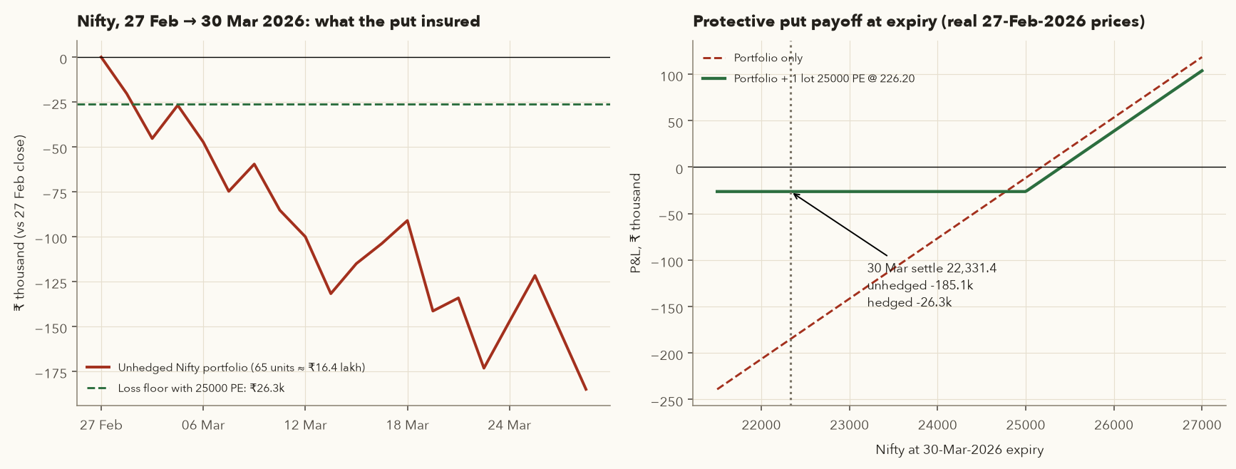
Suppose on 27 Feb 2026 you held a Nifty-tracking portfolio equal to one lot: 65 × 25,178.65 = ₹16,36,612. India VIX was a calm 13.70.
- Buy one lot of NIFTY 30-Mar-2026 25000 PE at 226.20 (real close, 96,294 contracts traded). Cost = 226.20 × 65 = ₹14,703, which is 0.898% of the portfolio for one month.
- Maximum loss at expiry = (25,178.65 − 25,000) + 226.20 = 404.85 points = ₹26,315 (1.61%), however far the market falls.
- What happened: Nifty fell 11.31% and settled at 22,331.40 on 30 Mar 2026 (expiry day, VIX 27.89).
- Portfolio: (22,331.40 − 25,178.65) × 65 = −₹1,85,071.
- Put: intrinsic = 25,000 − 22,331.40 = 2,668.60 points, so it pays ₹1,73,459. Net of premium the put made +₹1,58,756.
- Hedged result: −₹26,315, exactly the maximum loss computed in step 2, against −₹1,85,071 unhedged.
Futures variant. A trader long the March future at 25,338.60 instead lost 3,007.20 points (₹1,95,468) when it settled at 22,331.40. With the same put the loss would have been ₹36,712. The extra 160 points came from paying the futures premium over spot (Chapter 9).
Honest framing. In most months this insurance expires worthless. In the 24-month study in Section 11 the ATM put lost money in 13 of 24 months. You buy it for the months like March 2026, and you should size it so that the "wasted" premiums are an acceptable running cost.
Protecting a stock holding, and what happens at expiry
- 27 Feb 2026: you own 500 RELIANCE (one lot) at 1,393.90. Buy the 30-Mar 1380 PE at 21.45 (3,674 contracts traded). Cost ₹10,725, which is 1.54% of the position.
- Floor = (1,380 − 1,393.90 − 21.45) × 500 = −₹17,675.
- 30 Mar 2026 (expiry): RELIANCE settled at 1,343.90. The stock lost ₹25,000. The put is ITM by 36.10, and the net result is −₹17,675, the floor.
- Settlement is physical. An ITM long put on a stock means you deliver 500 shares and receive the strike, ₹6,90,000. Because you own the shares, the obligation is covered: the shares in your demat account are delivered and the position closes at 1,380. If you did not own them, you would have to buy them or face short-delivery penalties.
- STT on exercise is charged on intrinsic value (0.15% from 1 Apr 2026: 36.10 × 500 × 0.15% ≈ ₹27; it was 0.125% ≈ ₹22.56 at the time of this March expiry), plus delivery STT of 0.1% on the ₹6.9 lakh settlement value (₹690). Brokers also charge more for physical delivery: Zerodha, for example, charges 0.25% of the delivery value, about ₹1,725 plus GST here. If you want to keep the shares, sell the put before expiry instead of letting it exercise. On 30 Mar it closed at 38.10.
Sizing an index hedge for a stock portfolio
Most investors do not hold "the Nifty". To hedge a portfolio with Nifty puts, scale by its beta (Chapter 9):
- Portfolio value
- The current market value of your stock portfolio, in ₹.
- \(\beta\)
- The portfolio's beta: how much it tends to move for a 1% move in Nifty. 1.1 means about 1.1% (Chapter 9).
- Index level
- The current Nifty level, in points.
- Lot size
- Units per Nifty option contract (65).
How it works: the top line is the Nifty exposure your portfolio really carries (value scaled up or down by beta). The bottom line is the exposure covered by one lot of puts. Dividing gives the number of lots that matches the two. The answer is rarely a whole number, so you have to round up (over-hedge) or down (under-hedge).
Example: a ₹10,00,000 portfolio with beta 1.1 needs 10,00,000 × 1.1 / (22,620.45 × 65) = 0.748 lots. You cannot buy 0.748 lots, so one lot over-hedges (₹14.7 lakh notional) and zero leaves you unhedged. One 27-Oct 22000 PE cost 98.15 × 65 = ₹6,379.75 (0.64% of the portfolio). Lot granularity is a real practical limitation for small portfolios, and beta itself is unstable, so the protection is approximate.
Futures holder, today's prices: long one October Nifty future at 22,707.30 plus the 27-Oct 22300 PE at 161.70 (₹10,510.50) caps the loss to expiry at 22,707.30 − 22,300 + 161.70 = 569.00 points = ₹36,985 per lot, whatever happens overnight.
10.2 Covered call: earning a little on shares you hold
- \(S_0\)
- The share price when you sell the call.
- \(K\)
- The call's strike, above \(S_0\): the price at which your shares are effectively sold if the stock finishes above it.
- \(C\)
- The call premium you receive, in ₹ per share.
- Downside breakeven
- The expiry price below which the combined position starts losing money.
How it works: if the stock ends above the strike, you gain the rise up to the strike plus the premium you kept, and nothing more. If it falls, the premium covers only the first \(C\) rupees of the fall. Below \(S_0 - C\) you lose almost exactly as an unhedged holder would. Multiply by the lot size (500 for RELIANCE) for rupees.
The logic. You sell someone the upside beyond a strike in exchange for cash now. It suits a stock you are happy to hold but do not expect to rally sharply within the month. It is not a hedge in any serious sense, because the premium cushions only a small fall.
Covered call on 500 RELIANCE at 1,187
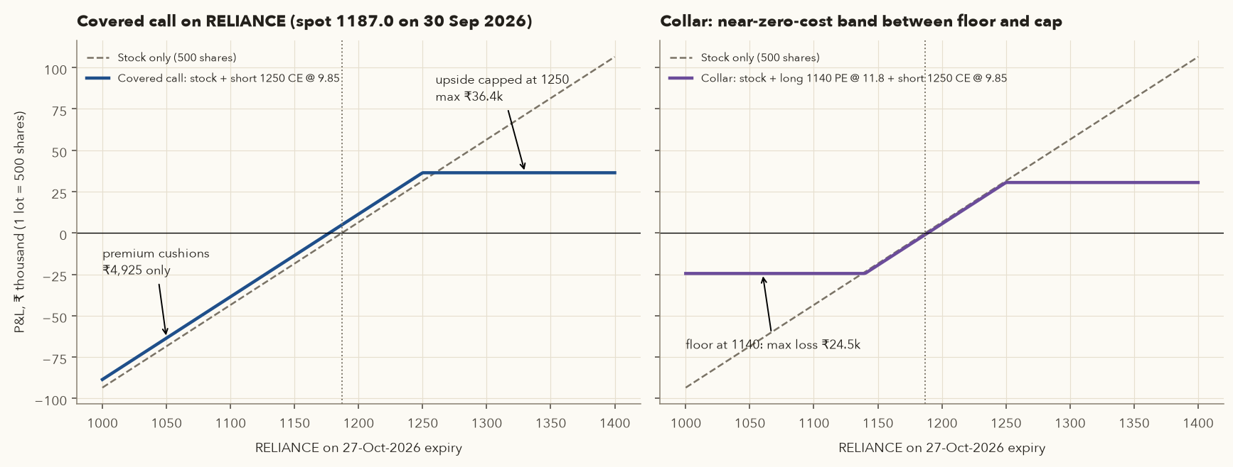
- Sell one lot of 27-Oct 1250 CE at 9.85 (14,567 contracts traded; 1250 is 5.31% above spot). Income = 9.85 × 500 = ₹4,925, which is 0.83% of the ₹5,93,500 holding.
- Max profit if RELIANCE ≥ 1,250 at expiry = (1,250 − 1,187 + 9.85) × 500 = ₹36,425. Above 1,250 your shares are effectively sold at 1,250 (physical settlement).
- Downside breakeven = 1,187 − 9.85 = 1,177.15. Below that you lose almost as much as an unhedged holder.
- Context from RELIANCE's own history (2016–Aug 2026, about 19-trading-day windows): it rose more than 5.31% in such a window 27.7% of the time. Roughly one month in four, the covered call would have given away upside.
Annualising 0.83% for 27 days (× 365/27) to "11.2% a year" is misleading. The occasional large rally you give up and the full downside you keep are what matter.
10.3 Collar: a floor paid for with a cap
- \(S_0\)
- The share price when you set up the collar.
- \(K_{put}\)
- The strike of the put you buy, below \(S_0\): your floor.
- \(K_{call}\)
- The strike of the call you sell, above \(S_0\): your cap.
- \(P,\ C\)
- The put premium you pay and the call premium you receive, in ₹ per share.
- \(P - C\)
- The net cost of the collar. Close to zero is a "zero-cost collar". If the call brings in more than the put costs, it is negative (a net credit).
How it works: the worst case is the stock falling to the floor, plus the net cost. The best case is the stock rising to the cap, minus the net cost. Between the two strikes you simply gain or lose with the stock. Multiply by the lot size for rupees.
A near-zero-cost collar
- Own 500 RELIANCE at 1,187. Buy the 1140 PE at 11.80 and sell the 1250 CE at 9.85. Net cost = 11.80 − 9.85 = 1.95 per share (₹975 per lot).
- Floor at 1,140 (3.96% below spot). Max loss = (1,187 − 1,140 + 1.95) × 500 = ₹24,475.
- Cap at 1,250. Max gain = (1,250 − 1,187 − 1.95) × 500 = ₹30,525.
- Historically RELIANCE fell more than 3.96% in about 19 trading days 21.6% of the time, and rose more than 5.31% 27.7% of the time. The collar caps both tails.
When to use it: you want to keep a long-term holding (for tax or conviction reasons) but get through a risky month, such as results or a big policy event, with a defined worst case. The cost is giving up upside in that window.
10.4 Bull call spread and bear put spread: cheaper directional views with defined risk
- \(K_1\)
- The strike of the option you buy, usually at or near the money.
- \(K_2\)
- The strike of the option you sell, further out of the money: above \(K_1\) for the bull call, below it for the bear put.
- CE, PE
- Call option and put option, as NSE labels them.
- \(D\)
- The net debit: premium paid for the bought option minus premium received for the sold one, in points.
- \(K_2 - K_1\), \(K_1 - K_2\)
- The distance between the strikes, in points: the most the spread can ever be worth at expiry.
- \(BE\)
- The breakeven level at expiry.
- Subtract the sold option's premium from the bought option's premium. That is \(D\), and it is the most you can lose.
- The spread is worth at most the gap between the strikes. Take away what you paid to get the maximum profit.
- The breakeven is the bought strike moved by \(D\): up for the bull call, down for the bear put.
- All figures are per unit. Multiply by the lot size (65 for Nifty) for rupees.
The logic: selling the further strike gives up profits beyond it in exchange for cutting the cost, the delta and, most importantly, the theta and vega of the position. For a hedger, a bear put spread is a cheaper partial hedge. It covers a moderate fall (say 2–4%) but not a crash beyond the lower strike.
Spreads vs naked options
| Bull call 22600/23000 | Naked 22600 CE | Bear put 22600/22200 | Naked 22600 PE | |
|---|---|---|---|---|
| Net debit (points) | 372.90 − 177.80 = 195.10 | 372.90 | 258.05 − 135.50 = 122.55 | 258.05 |
| Max loss / lot | ₹12,681.50 | ₹24,238.50 | ₹7,965.75 | ₹16,773.25 |
| Max profit (points) | 400 − 195.10 = 204.90 | unlimited | 400 − 122.55 = 277.45 | ≈ strike − premium |
| Max profit / lot | ₹13,318.50 | — | ₹18,034.25 | — |
| Breakeven | 22,795.10 | 22,972.90 | 22,477.45 | 22,341.95 |
| Delta (at own IVs) | 0.206 | 0.563 | −0.174 | −0.437 |
| Theta (pts/day) | −1.26 | −7.60 | −0.04 | −4.19 |
The bull call spread's theta is about one-sixth of the naked call's and its vega is 1.29 against 24.24. Time and volatility hurt it much less, and the price of that is a capped payoff. This is Varsity's main argument for spreads over naked buying when your view is "moderately up" or "moderately down".
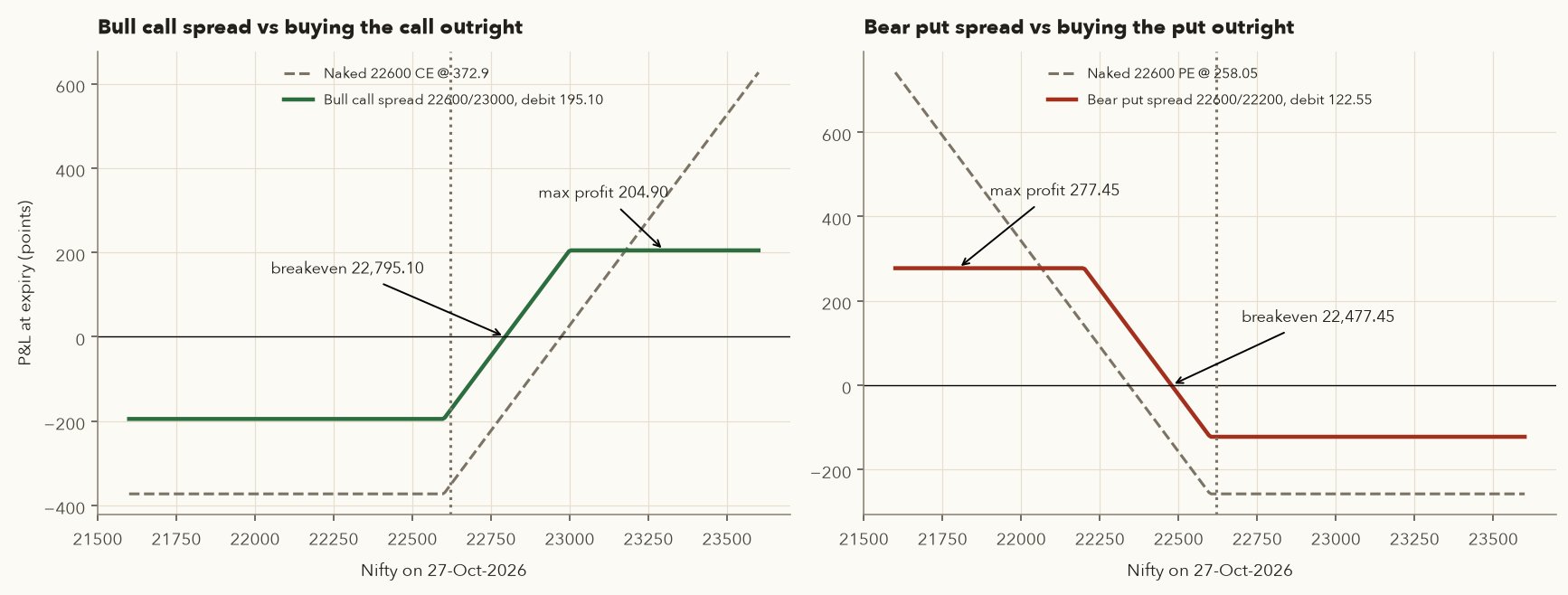
Strike selection for spreads (Varsity's guidance, in brief): if you expect the move within a few days, early in the series, both strikes can be OTM. If you expect it by expiry, buy ATM and sell OTM. Late in the series, move the bought strike ITM or ATM because theta punishes OTM legs. Volatility matters less for spreads early in the series and more near expiry.
- Must survive a crash, can afford premium: protective put, preferably a month or longer (cheaper per day), bought when IV is calm.
- Want protection with almost no cash outlay, accept a cap: collar.
- Only worried about a moderate dip: bear put spread.
- Want income, accept full downside: covered call. It is not a hedge.
- Short futures, fear a squeeze: buy a call (the mirror of the protective put).
11. Why option buying mostly loses, and why selling has tail risk
Buyers lose most of the time, because of time decay, slightly overpriced volatility and trading short-dated options. Sellers win most months but can lose many months of income in one crash. Neither side gets an easy edge. Use options to define and reduce risk, not as lottery tickets.
11.1 What SEBI's data says
SEBI's study "Profitability of Individual Traders in the Equity Derivatives Segment (FY25–FY26)", released in August 2026, found that the share of losing individual traders was 87.7% in FY26, down from about 91% in FY25. The average loss was about ₹1.17 lakh per trader, nearly 97% of traders predominantly bought options, and individuals paid about ₹25,000 crore in transaction costs in FY26. Before costs, 82.1% were already loss-making, so charges alone turned roughly another 5.6% of all traders from a gross gain into a net loss. Trading was crowded into the last moments of a contract's life: about 59% of index-option turnover was in contracts expiring that same day ("zero days to expiry"), 75% within one day and 97% within a week. That is exactly where theta and gamma are most extreme (Section 7). The earlier study (FY22–FY24) found 93% of over one crore individual traders lost money. FY25 net losses were first reported at ₹1,05,603 crore in SEBI's July 2025 study and revised to about ₹1,11,788 crore in the 2026 study. The pattern holds year after year.
11.2 Why buyers lose: three forces against them
- Theta. The option loses value every day the move does not happen. A buyer must be right about direction and size and timing.
- The volatility risk premium. Implied vol is usually above what is later realised (81.1% of days since 2016, Section 8.2), so options are on average slightly overpriced.
- Behaviour and costs. Most retail activity is in near-expiry OTM options: cheap tickets with low probability that decay fastest. Brokerage, STT (now 0.15% of premium on sales) and spreads take a larger share of a small premium.
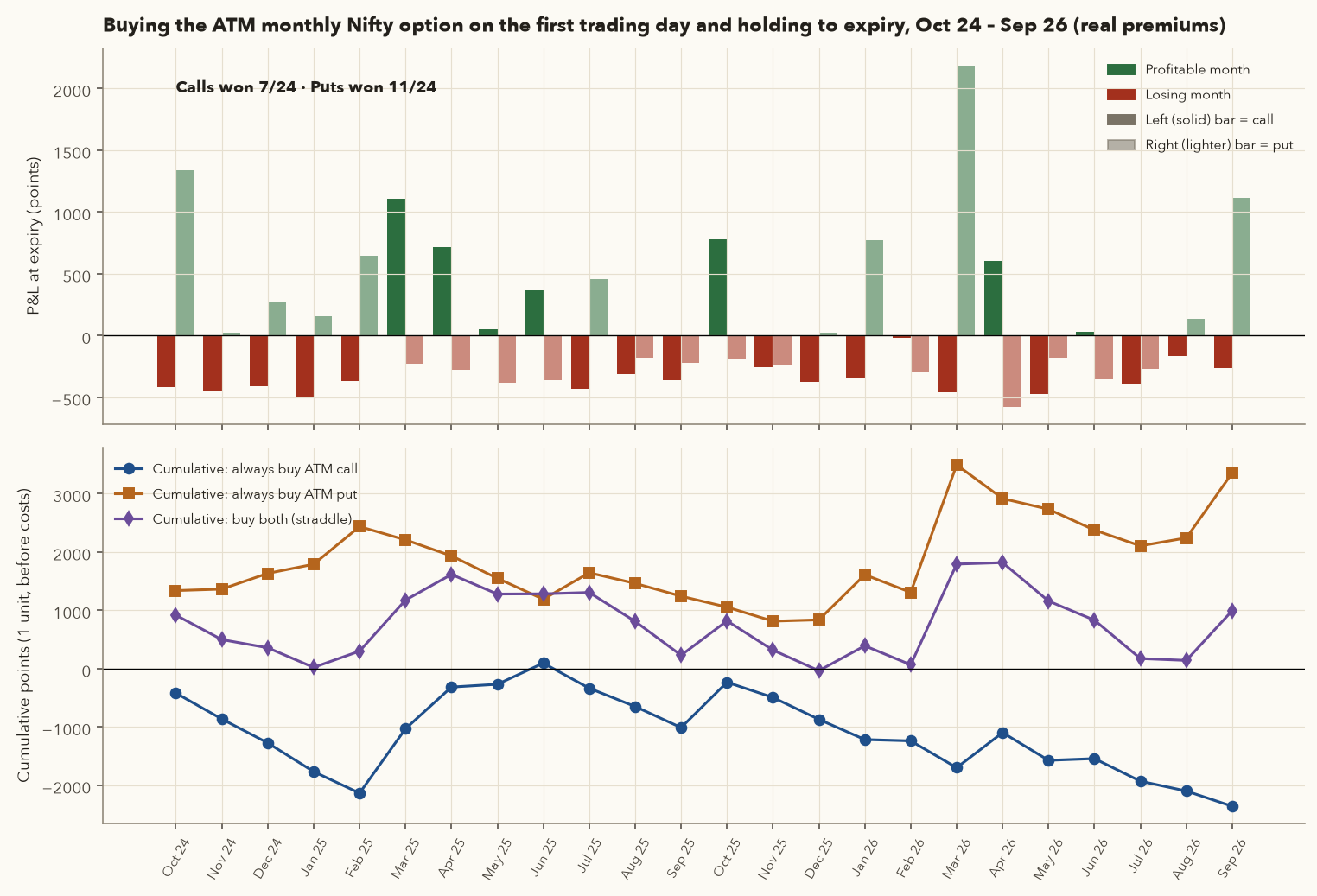
Buy the ATM monthly call and put on the first trading day, hold to expiry
Using actual NSE closing premiums on the first trading day of each month (24 months), with the payoff at the monthly expiry:
| ATM call buyer | ATM put buyer | Both (straddle) | |
|---|---|---|---|
| Months won | 7 / 24 | 11 / 24 | 11 / 24 |
| Expired worthless (lost 100%) | 14 | 10 | — |
| Total P&L, points (before costs) | −2,362.4 | +3,355.2 | +992.8 |
| Best month | +1,103.8 (Mar 2025) | +2,186.4 (Mar 2026) | +1,726.7 (Mar 2026) |
Honest reading. Most individual trades lost (17 of 24 call trades, 13 of 24 put trades), but this particular window included two sharp falls: Nifty went from 25,796.90 at the start to 22,620.45 at the end. Put buyers made money overall, mostly from a few big months: March 2026, October 2024 and September 2026 together contributed 4,637.75 points. The average straddle cost 704.38 points against an average absolute move at expiry of 745.75, so buyers were slightly ahead in this window. Short samples can show anything, so we also need a longer test.
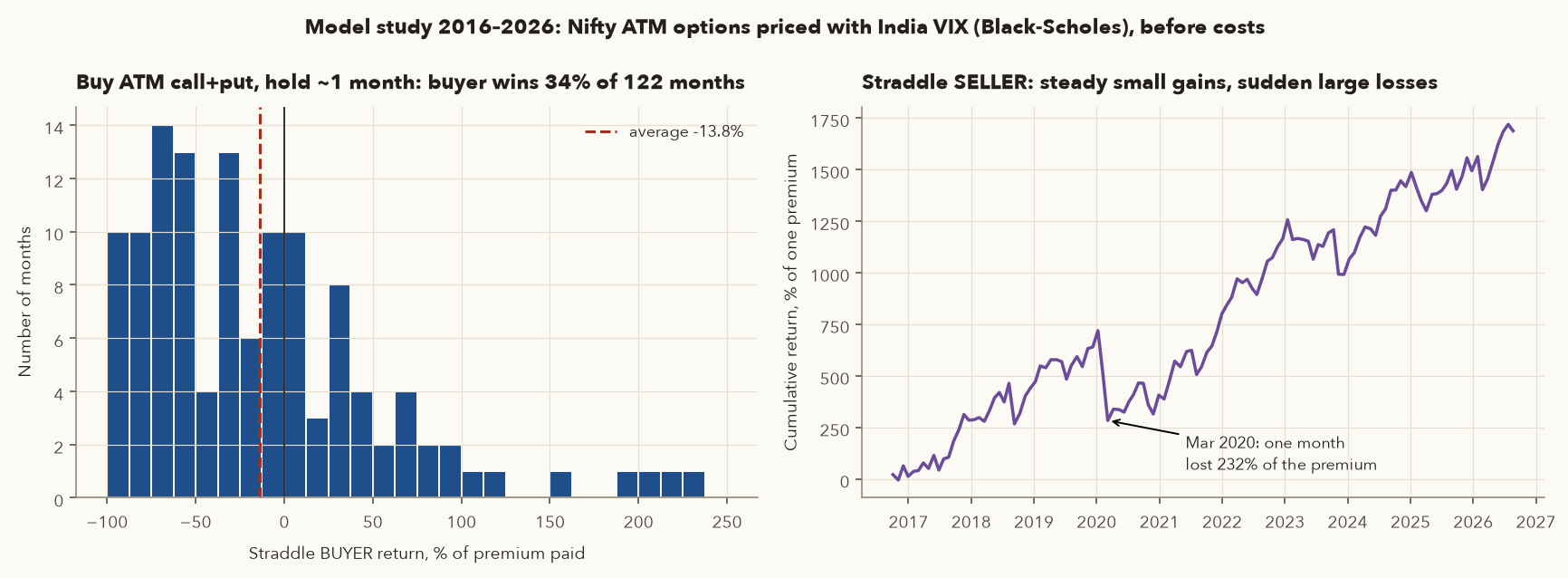
Ten years of buying straddles
We have no option prices for every month back to 2016, so this test models each premium with Black-Scholes at that day's India VIX. Because VIX usually sits a little above the ATM IV (Section 6.3), the model somewhat overstates premiums, so read the results as indicative.
- Monthly (20-trading-day) ATM straddle, 122 months: the buyer won only 34.4% of months. The average result was −13.8% of the premium and the median −31.6%. Calls alone won 40.2% and puts alone 22.1%.
- Weekly (5-day) straddle, 489 weeks: the buyer won 35.8%, with an average of −12.0%.
- The seller's worst month began 6 Mar 2020: a loss of 231.7% of the premium collected (381.7% on the weekly version). One bad month wiped out many months of gains.
11.3 Why sellers get hurt: the tail
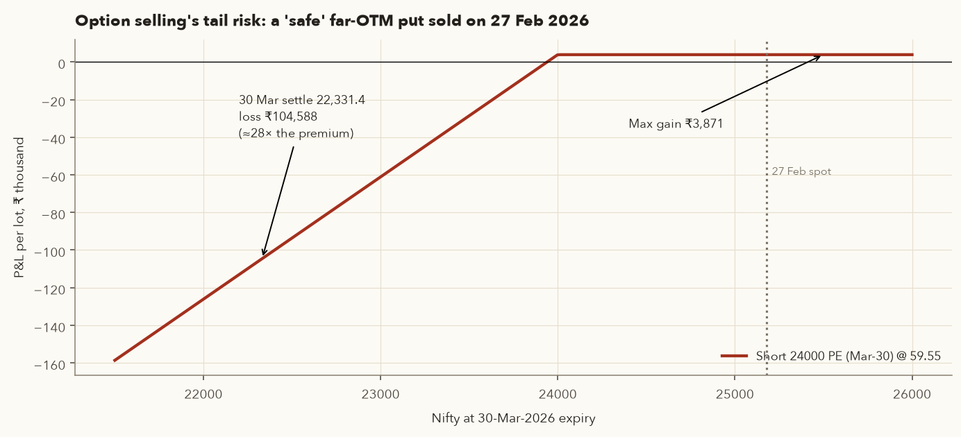
The "safe" far-OTM put
- 27 Feb 2026: Nifty 25,178.65, VIX 13.70. The 24000 PE (4.7% OTM) traded at 59.55. Selling one lot collected ₹3,871. It looked like easy money.
- 30 Mar 2026: Nifty settled at 22,331.40. The put's intrinsic value was 24,000 − 22,331.40 = 1,668.60.
- Seller's loss = (1,668.60 − 59.55) × 65 = ₹1,04,588, about 27× the premium collected (the seller had to pay out 28× the premium and had pocketed 1×). Margin calls would have arrived all month as the premium rose and VIX doubled.
This is the core asymmetry. Sellers win most months (Section 5's "zone"), but their payoff distribution has a fat left tail. Without a hedge such as a bought further-OTM put (turning the trade into a spread), one tail event can erase years of income.
- Use options mainly to reduce risk (protective puts, collars, defined-risk spreads), not to gamble on near-expiry moves.
- If you buy for direction, buy time: monthly options, not same-day ones. Use spreads to cut theta, and size so that losing 100% of the premium is acceptable.
- If you ever sell options, never sell naked without a defined-loss hedge, and size for the March 2020 / March 2026 month, not the average month.
12. Settlement, expiry, margins and costs (verified Oct 2026)
12.1 What happens at expiry
- Index options (Nifty): cash-settled. ITM options are automatically exercised at the final settlement price, the index close on expiry day. On 30 Mar 2026 every March Nifty option settled against 22,331.40. The 25000 PE's closing price that day was 2,682.90, but it settled at its intrinsic value, 2,668.60, and that is what holders received. OTM options expire worthless.
- Stock options: physically settled (mandatory for all stock F&O since October 2019). ITM long call: you buy the shares at the strike. ITM long put: you deliver the shares and receive the strike. Short positions have the mirror obligations. You need the full cash or the shares, not just margin.
- Opposite ITM positions in the same stock and expiry (for example long futures and a long ITM put) are netted, and only the difference is delivered.
Margins rise as stock-option expiry approaches (expiry on Tuesday)
| Day | Long stock options (ITM contracts; on expiry day also OTM strikes very close to spot) |
|---|---|
| E−4 (Wednesday) | 10% of exchange risk margins (VaR + ELM + ad hoc: the value-at-risk margin, the extreme-loss margin and any special margin the exchange adds) |
| E−3 (Thursday) | 25% of those margins |
| E−2 (Friday) | 45% of those margins |
| E−1 (Monday) | 25% of contract value |
| Expiry (Tuesday) | 50% of contract value for ITM; 25% for OTM strikes very close to spot (within 1% for stocks above ₹100) |
Short stock options: on expiry day, 50% of contract value or 1.5× normal (NRML) margin, whichever is lower. Either way, for any stock-option position that may finish ITM, plan to have close to its full delivery value (cash for a buyer of shares, shares for a seller) available by expiry. Positions without enough margin may be squared off by the broker (with a charge). The client remains responsible for closing positions. Other brokers have similar, not identical, rules, so check yours.
12.2 Margins and upfront premium
- Buyers pay the full premium upfront. There is no mark-to-market, and the maximum loss is the premium. SEBI's October 2024 framework made upfront collection of net option premium mandatory at client level.
- Sellers post SPAN margin (the exchange's estimate of the worst one-day loss across a set of price and volatility scenarios) plus exposure margin (an extra safety buffer), of the same order as a futures margin (for a Nifty lot, typically well over ₹1 lakh; use your broker's margin calculator for the live figure). Margin rises when the premium or volatility moves against you, which can force exits at the worst time. Hedged positions such as spreads need much less margin.
- SEBI measures in force since late 2024 / early 2025: an extra 2% extreme-loss margin on short index options on expiry day, no calendar-spread margin benefit on expiry day, intraday monitoring of position limits, and a minimum contract value of ₹15 lakh at the time of lot-size reviews. Note that one Nifty lot (65 units) was worth only ₹14.70 lakh on 30 Sep 2026 after the fall, which is why exchanges revise lot sizes periodically.
12.3 Costs and STT (from 1 Apr 2026)
| Charge | Rate | Note |
|---|---|---|
| STT on option sale | 0.15% of premium | Raised from 0.1% in Union Budget 2026, effective 1 Apr 2026 |
| STT on exercised ITM options | 0.15% of intrinsic (settlement) value | Was 0.125% before 1 Apr 2026 |
| STT on futures sale | 0.05% | Was 0.02% before 1 Apr 2026 |
| Physically settled stock options | Delivery STT 0.1% on settlement value (buyer and seller) | As for delivery trades |
Example: selling one lot of the 22600 CE at 372.90 incurs STT of 372.90 × 65 × 0.15% = ₹36.36, plus brokerage, exchange charges, SEBI fees, stamp duty and GST. Chapter 13 computes the full stack and the tax treatment: F&O profits are normally taxed as non-speculative business income.
13. Try it yourself
These snippets need a copy of the course repository and Python with pandas and numpy (setup steps are in its framework/README.md). Run them from the repository's root folder, for example with .venv/bin/python, because the file paths are relative to that folder. Each reproduces numbers from this chapter.
(a) Intrinsic/time value, PCR and max pain from the real chain
import pandas as pd
chain = pd.read_csv("data/fno/nifty_options_2026-09-30.csv", parse_dates=["XpryDt"])
spot = chain.UndrlygPric.iloc[0]
oct27 = chain[chain.XpryDt == "2026-10-27"]
ce = oct27[oct27.OptnTp == "CE"].set_index("StrkPric")
pe = oct27[oct27.OptnTp == "PE"].set_index("StrkPric")

for k in [22200, 22600, 23000]:
    c_iv, p_iv = max(0, spot - k), max(0, k - spot)
    print(k, "CE", ce.loc[k, "ClsPric"], "TV", round(ce.loc[k, "ClsPric"] - c_iv, 2),
          "| PE", pe.loc[k, "ClsPric"], "TV", round(pe.loc[k, "ClsPric"] - p_iv, 2))

print("PCR:", round(pe.OpnIntrst.sum() / ce.OpnIntrst.sum(), 3))      # 1.012

def pain(x):
    k_c, k_p = ce.index.to_numpy(), pe.index.to_numpy()
    return ((x - k_c).clip(min=0) * ce.OpnIntrst.to_numpy()).sum() + \
           ((k_p - x).clip(min=0) * pe.OpnIntrst.to_numpy()).sum()
strikes = sorted(set(ce.index) | set(pe.index))
print("Max pain:", min(strikes, key=pain))                             # 23400
(b) Black-Scholes and implied volatility
import numpy as np
from scipy.stats import norm
from scipy.optimize import brentq

def bs_call(S, K, T, sigma, r=0.054):
    d1 = (np.log(S / K) + (r + sigma**2 / 2) * T) / (sigma * np.sqrt(T))
    d2 = d1 - sigma * np.sqrt(T)
    return S * norm.cdf(d1) - K * np.exp(-r * T) * norm.cdf(d2), norm.cdf(d1)

S, K, T = 22620.45, 22600, 27 / 365
price, delta = bs_call(S, K, T, 0.1349)        # India VIX as vol -> 388.48, delta 0.56
iv = brentq(lambda s: bs_call(S, K, T, s)[0] - 372.90, 0.01, 2)
print(round(price, 2), round(delta, 3), "IV", round(iv * 100, 2), "%")   # IV 12.85 %
(c) Hedge payoffs on RELIANCE at expiry (₹ per lot)
spot, put_k, put_prem, call_k, call_prem, lot = 1187.0, 1140, 11.80, 1250, 9.85, 500
for x in [1050, 1100, 1140, 1187, 1250, 1300]:
    stock = x - spot
    protective = stock + max(0, put_k - x) - put_prem
    covered = stock + call_prem - max(0, x - call_k)
    collar = stock + max(0, put_k - x) - put_prem + call_prem - max(0, x - call_k)
    print(x, stock * lot, round(protective * lot), round(covered * lot), round(collar * lot))
# at 1050: stock -68,500 | protective put -29,400 | covered call -63,575 | collar -24,475
Every chart in this chapter is reproduced by course/scripts/ch10_figures.py. The NSE bhavcopy extracts it needs are downloaded by course/scripts/ch10_data.py.
Use framework.data.load_option_chain() to load the latest Nifty chain, and framework.futures.beta_hedge(portfolio_value, beta, fut_price, lot) for the beta-scaled lot count (the same formula works for index puts). Price a hedge's full cost with framework.costs.options_charges and size the underlying position with framework.risk.position_size, counting the put's max loss as your risk. The Black-Scholes and implied-vol helpers from snippet (b) are worth keeping in your own utilities module. The framework API does not include an options pricer.
14. Practical checklist
Before using an option to hedge
- ☐ What exactly am I protecting against (gap on results, event, crash), and for how long?
- ☐ What maximum loss do I accept? Strike = entry − acceptable loss, before premium.
- ☐ Expiry: does it cover the risk window, with a margin of safety? Longer expiries cost less per day.
- ☐ Is IV calm or elevated? (Check India VIX and the strike's IV vs its recent history.) Avoid buying protection in a panic if you can plan ahead.
- ☐ Cost as % of the position, per month. Is that an acceptable running cost if nothing happens?
- ☐ Would a spread or collar give enough protection more cheaply?
- ☐ Liquidity: volume and OI at the strike, and a tight bid-ask. Use limit orders.
- ☐ Size: index hedge lots = value × beta / (index × lot). Check the over- or under-hedge from rounding.
- ☐ Stock options: the physical-settlement plan. Close before expiry week, or have the shares/cash ready. Know your broker's E−4 to E margin schedule.
- ☐ Costs: STT 0.15% on premium sold / intrinsic exercised (from 1 Apr 2026), plus other charges.
Before any directional option trade
- ☐ Breakeven computed. How far and how fast must the market move?
- ☐ Delta, theta and vega understood. What do I lose per day if nothing happens?
- ☐ Losing 100% of the premium is acceptable within my risk-per-trade rule (Chapter 11).
- ☐ No naked short options. Any short leg has a defined-risk hedge.
- ☐ Not trading same-day-expiry contracts "because they're cheap".
15. Key takeaways
- A call is the right to buy and a put the right to sell at the strike. Buyers pay a premium for a capped loss, and sellers collect it in exchange for a large or unlimited loss.
- Premium = intrinsic + time value. Time value peaks at the money and decays towards zero, fastest in the last week.
- Breakevens: long call K + C, long put K − P. On 30 Sep 2026 the 22600 call needed Nifty above 22,972.90 by 27 Oct.
- Black-Scholes is a ruler, not truth. Inverting it gives implied volatility, which differs by strike (the skew: downside puts are dearer).
- Delta (direction), gamma (change in delta), theta (time) and vega (volatility) together explained a real one-day move to within 0.2 points.
- India VIX implied a ±830-point (1 SD) Nifty range to the 27-Oct expiry. Implied vol has exceeded realised vol on about 81% of days since 2016, and that gap is the sellers' edge.
- OI, PCR and max pain are context, not signals. The monthly max pain was 800 points from spot on 30 Sep 2026.
- A protective put turned a ₹1,85,071 loss into ₹26,315 in March 2026, at a cost of ₹14,703. In most months the same premium is simply lost.
- A collar trades upside for a cheap floor. Spreads cut cost, theta and vega in exchange for capped gains. A covered call is income, not a hedge.
- SEBI: 87.7% of individual F&O traders lost money in FY26, and ~92% of losses came from options. A far-OTM put sold for 59.55 in Feb 2026 lost about 27× its premium a month later.
- Stock options are physically settled. Know your broker's expiry-week margins. STT rose to 0.15% on options from 1 Apr 2026.
16. Quiz and exercises
Q1. On 30 Sep 2026, Nifty was 22,620.45. Classify the 22400 CE and the 22400 PE by moneyness, and split the CE's premium of 501.15 into intrinsic and time value.
Q2. You sell one lot of the 27-Oct 22600 PE at 258.05. What is your breakeven, your maximum profit in rupees, and your P&L if Nifty settles at 21,800?
Q3. A call has delta 0.56, gamma 0.00048, theta −7.88 and vega 24.26. Estimate the premium change over one day if Nifty rises 100 points and IV falls by 1 point.
Q4. Using India VIX = 13.49% and spot 22,620.45, compute the 1-SD expected move over 6 calendar days (to the 06-Oct weekly). Compare it with the weekly ATM straddle price of 279.15.
Q5. You hold a ₹25,00,000 stock portfolio with beta 0.9. How many Nifty lots of puts would hedge it at Nifty 22,620.45 and lot 65? What practical problem appears?
Q6. Build a bear put spread from the 27-Oct 22600 PE (258.05) and 22200 PE (135.50). Give the net debit, max profit, max loss per lot and breakeven. Why might a hedger prefer it to the naked put?
Q7. You are long 500 RELIANCE and long the 1380 PE. On expiry RELIANCE closes at 1,343.90. What happens to your shares if you do nothing, and what should you do if you want to keep them?
Q8. A friend says: "Selling far-OTM puts is safe. They expire worthless 90% of the time." Use the Feb–Mar 2026 example to explain the flaw.
Q9. Why did the 90-day 22600 PE cost only about 3.3× the 6-day 22600 PE, and what does that imply for someone hedging a portfolio for three months?
Q10. The 27-Oct monthly max pain was 23,400 with spot at 22,620.45. Should you expect Nifty to drift up to 23,400 by expiry? Explain.
Exercise. Using data/extra/ch10_options_20260227.csv, price a collar on a Nifty portfolio for March 2026: buy the 24500 PE and sell the 26000 CE (30-Mar-2026 expiry). What was the net cost, and what would the hedged result have been at the 22,331.40 settlement?
TckrSymb=="NIFTY" and XpryDt=="2026-03-30", then read ClsPric: the 24500 PE closed at 115.30 and the 26000 CE at 100.40. Net cost = 115.30 − 100.40 = 14.90 points (₹968.50 per lot). At the 22,331.40 settlement the put is ITM and the call expires worthless, so the hedged loss per unit = (25,178.65 − 24,500) + 14.90 = 693.55 points = ₹45,080.75, against ₹1,85,071 unhedged. The price of the near-free floor was giving up any gain above 26,000. Compare this with the 25000 protective put (₹26,315 loss, ₹14,703 premium): a cheaper hedge with a lower floor.17. Sources
Primary concepts (explained here in our own words): Zerodha Varsity Module 5, Options Theory for Professional Trading:
Ch 1 Call Option Basics ·
Ch 2 Basic Option Jargons ·
Ch 3 Buying a Call Option ·
Ch 4 Selling/Writing a Call Option ·
Ch 5 The Put Option Buying ·
Ch 6 The Put Option Selling ·
Ch 7 Summarizing Call & Put Options ·
Ch 8 Moneyness ·
Ch 9–11 Delta ·
Delta Part 3 ·
Ch 12–13 Gamma ·
Ch 14 Theta ·
Ch 15 Volatility Basics ·
Ch 16 Volatility Calculation ·
Ch 17 Volatility & Normal Distribution ·
Ch 18 Volatility Applications ·
Ch 19 Vega ·
Ch 20 Greek Interactions ·
Ch 21 Greek Calculator ·
Ch 22 Re-introducing Call & Put Options ·
Ch 24 Physical Settlement ·
Ch 25 Options M2M and P&L.
Zerodha Varsity Module 6, Option Strategies:
Orientation ·
Bull Call Spread ·
Synthetic Long & Arbitrage ·
Bear Put Spread ·
Max Pain & PCR Ratio.
(Varsity has no dedicated protective-put, covered-call or collar chapters. Those sections combine the payoff logic of Module 5 with the hedging ideas in Module 4 and Module 9.)
Rules and statistics (verified Oct 2026):
Zerodha: policy on physical settlement of equity derivatives ·
Zerodha Z-Connect: physical delivery of stock F&O ·
SEBI circular SEBI/HO/MRD/TPD-1/P/CIR/2024/132 (1 Oct 2024), measures to strengthen the equity index derivatives framework ·
NSE circular: revision in expiry day of index derivatives ·
Nifty lot size revised to 65 (Jan 2026 series) ·
STT rates after Union Budget 2026 (effective 1 Apr 2026) ·
SEBI FY26 study coverage (87.7% lost, ₹91,685 crore) ·
SEBI study release, 20 Aug 2026 ·
SEBI FY26 study: 92% of losses from options, 59% same-day-expiry turnover (Moneylife) ·
SEBI FY25 study (Business Standard, Jul 2025) ·
SEBI FY22–FY24 study (Business Standard, Sep 2024) ·
NSE holiday calendar 2026.
Data: NSE F&O UDiFF bhavcopies for 27-Feb-2026, 30-Mar-2026, 30-Sep-2026 and the first trading day of each month Oct 2024–Sep 2026 (nsearchives.nseindia.com), saved under data/extra/ch10_*.csv. Nifty option chain and futures: data/fno/. Nifty 50 and India VIX daily history: NSE via Yahoo Finance (data/ohlc/). Risk-free rate 5.4% approximates the 91-day T-bill yield in Sep 2026 (auction cut-offs ranged from about 5.2% to 5.5% that month; RBI repo held at 5.25% in the Aug 2026 policy). All computations: course/scripts/ch10_figures.py.