
Trading Systems & Backtesting
1. What you'll learn and why it matters
So far this course has given you tools: candlesticks, support and resistance, indicators, a swing playbook, fundamentals, futures, options and risk rules. A trading system combines those tools into one complete written rulebook, and backtesting checks how that rulebook would have done on past data before you put money behind it.
By the end of this chapter you will be able to:
- Write a complete system: universe, entry, exit, position size and risk limits, with no gaps left to "judgement on the day".
- Build a backtester in pandas yourself: signals at the close, fills at the next open, stops, Indian transaction costs, slippage and an equity curve.
- Calculate and interpret CAGR, volatility, Sharpe, Sortino, maximum drawdown, Calmar, win rate, profit factor, expectancy, average holding period and exposure.
- Judge three real systems tested on 2017–2026 NSE data: a Nifty 50/200 crossover, a 55-day breakout portfolio with 1% risk sizing, and RSI(2) mean reversion.
- Spot the six classic backtesting mistakes (look-ahead, survivorship, overfitting, ignoring costs, no out-of-sample test, small samples). Each one is shown on real data.
- Run both of Varsity's pair-trading methods (ratio + density curve, and regression + ADF test + z-score) on real Indian bank and IT pairs, plus Varsity's calendar-spread and momentum-portfolio systems.
- Move a system from backtest to paper trading to small live size with a checklist.
Swing traders: without a tested rulebook, every trade is a fresh guess and every loss feels like a disaster. With one, you know that a 20-trade losing streak can happen inside a system that still makes money (System B below had one). Long-term investors: the same tools tell you whether a "rule" such as "sell when the 50-day crosses below the 200-day" actually beats doing nothing. On Nifty it did not (Section 6). Future futures traders: with leverage, an untested system loses money quickly. The pair and calendar-spread sections use real futures lot sizes and current F&O charges.
Most of what you will see in this chapter is disappointing, on purpose. Two of our three systems lost to plain buy-and-hold after costs. The one that beat Nifty did so mainly because of the stocks we chose to test it on. Random entries with the same exits did as well as its breakout entries. That is a normal result. Backtesting is mostly a tool for rejecting bad ideas cheaply, before they cost real money. Everything here is historical analysis for learning, not a recommendation to buy or sell anything.
Sections 2–10 are the core: what a system is, how to backtest one honestly, and how to judge the result. Sections 11–13 (pair trading and calendar spreads) need futures and some statistics, so on a first read you can skim them and return after you are comfortable with Chapter 9. Section 14 (momentum portfolios) and Section 16 (going live) apply to everyone. Section 15 has short programs you can run yourself.
2. What a trading system is (and is not)
Varsity's Module 10 opens with a trade its author placed on 25 Oct 2017, the day after the government announced ₹2.1 lakh crore of recapitalisation for public-sector banks. PSU bank stocks shot up. Bank Nifty rose about 3%, even though PSU banks were only a small slice of that index. That looked overdone, so the author sold a Bank Nifty strangle to collect premium. Varsity calls this kind of reasoning systematic deduction: a sensible, one-off chain of logic. It is also not a system, because it cannot be written down as a repeatable process and tested on history. The same is true of trading on gut feel, on a friend's tip, on a TV anchor's call or on a broker's call.
A trading system is a process with defined inputs (prices, volumes, fundamentals), fixed logic, and an output that tells you what to do: trade or don't, how much, and when to get out. You design the logic once and then follow it. Varsity warns that a system is not a "holy grail" money machine. You still choose the inputs, design the logic and decide to follow it, so the results are still your responsibility.
The five parts of a complete system
| Component | Question it answers | Example (System B in this chapter) |
|---|---|---|
| Universe | Which instruments am I allowed to trade? | The 37 large, liquid NSE stocks in the course data set |
| Entry | Exactly when do I buy (or sell short)? | Close above the highest high of the previous 55 sessions; buy at the next day's open |
| Exit | When do I get out, whether I am winning or losing? | Close below the lowest low of the previous 20 sessions, or the initial stop is touched |
| Position size | How many shares or lots? | Risk 1% of current equity between entry and a 2×ATR(20) stop; never more than 20% of equity in one stock |
| Portfolio / risk rules | How much in total, and what if many signals come at once? | Maximum 10 open positions; if there are more signals than slots, take the strongest 6-month performers first |
If any of the five is missing, you will fill the gap with emotion at the worst possible moment. "I'll exit when it looks weak" is not an exit rule.
Discretionary vs systematic
| Aspect | Discretionary trader | Systematic trader |
|---|---|---|
| Decision | Reads the chart and context, decides on the day | Rules decide; the trader executes |
| Can it be backtested? | Not reliably (memory and hindsight leak in) | Yes, on years of data in minutes |
| Strength | Adapts to unusual events (results, policy, news) | Consistent; removes fear and greed from each decision; scales to many stocks |
| Weakness | Inconsistent; biases (Chapter 11) creep in; hard to tell skill from luck | Can be over-fitted to history; can fail when the market changes; boring to follow through losing streaks |
| Realistic middle ground | A rules-based trader: the system generates the candidates and fixes size and stop; discretion is allowed only to skip a trade for a written reason (for example, results due tomorrow), never to widen a stop or add size. | |
Varsity's module planned five systems (pair trading, volatility-based, delta hedging, calendar spreads, momentum). It finished three in detail: pair trading (two methods), calendar spreads and a momentum portfolio. Its author says plainly that he left out backtesting because he did not code, and that you must backtest any system yourself before trading it. This chapter fills that gap. It teaches the backtesting method, applies it to three common swing/positional systems, and then backtests Varsity's own three systems on 2026 data.
3. The design process: idea to live money
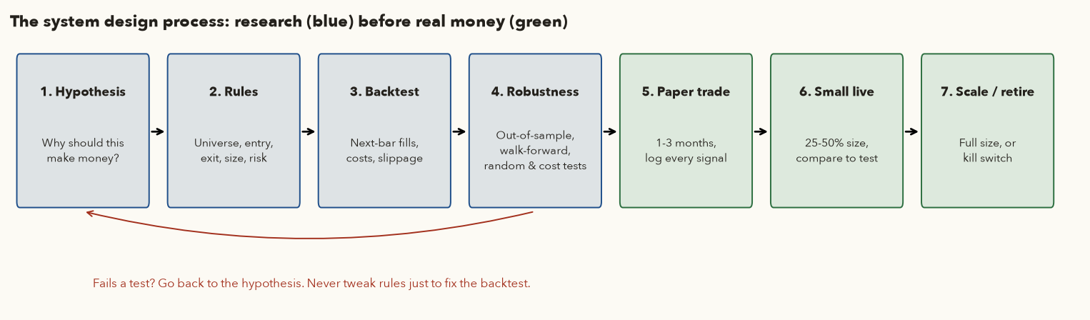
- Hypothesis: why should this make money? Write one sentence about market behaviour. "Stocks breaking to new highs tend to keep going because institutions buy in stages" is a hypothesis. "RSI below 30 is good" is not. If you cannot explain who is on the other side of the trade and why they lose, be suspicious of any profit you find.
- Rules. Turn the idea into the five components above, precisely enough that two people coding it would get the same trades. Decide the parameters before you look at results (use textbook defaults: 50/200, 55/20, RSI(2) < 10).
- Backtest. Run the rules on history with realistic execution (next-bar fills), costs and slippage.
- Robustness. Do the results survive a different period (out-of-sample), small changes in parameters, higher costs, random entries with the same exits, and a universe that includes the losers? Section 10 does each of these.
- Paper trade for 1–3 months. Log every signal in real time, exactly as the rules say. This catches practical problems a backtest cannot: missed orders, gaps at the open, data that arrives late, and your own reluctance to take a trade.
- Small live. Trade at 25–50% of the intended size for at least 20–30 trades and compare live results with the backtest's distribution.
- Scale up or retire. Go to full size only if live results fall inside the backtest's normal range. Set a kill switch in advance, for example "stop if drawdown exceeds 1.5× the backtest's maximum".
If a test fails, go back to step 1 with a new hypothesis. Do not tweak parameters until the backtest looks good. Every tweak "uses up" some of the history's information. After enough of them you have a perfect fit to the past and no edge in the future. Section 10.3 shows this on real data.
4. Build a backtester from scratch, step by step
A backtester answers one question: if I had followed these rules, trading only on information available at the time, what would my account have done? The phrase "only on information available at the time" is where most beginners' backtests go wrong. So we start with timing.
Two terms first. Slippage is the gap between the price your rules assume and the price you actually get (the bid-ask spread plus the price moving while your order fills). It is a hidden cost, so we charge a fixed percentage for it on every buy and sell. A vectorised backtest does each calculation on a whole column of dates at once (for example, one line computes the 50-day average for every day), instead of looping through the days one at a time. It is fast and short, and works well for one instrument that is either fully in or fully out.
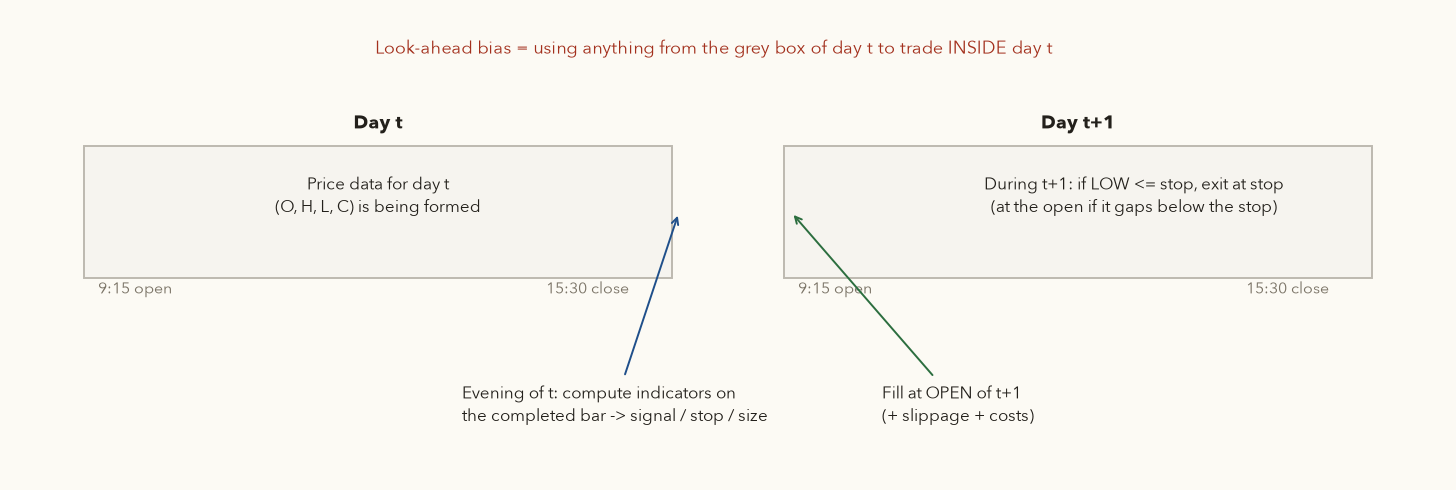
This convention suits swing and positional traders: you scan after 3:30 pm, place orders in the evening or before 9:15 am, and get filled at or near the open. It is also conservative. You never assume you got the signal day's closing price, because you only knew the signal after the close.
4.1 The six steps of a vectorised backtest (one instrument)
- Load clean data. Daily OHLC, split- and bonus-adjusted. (Our files are split-adjusted but not dividend-adjusted. For a price-index system on Nifty that is what you want.)
- Compute the signal at the close. For example
signal = SMA50 > SMA200. A value of 1 means "I want to be long from tomorrow". Every indicator may use only data up to and including today. - Shift by one bar to get the position.
position = signal.shift(1). This single line is the difference between an honest backtest and a fantasy (Section 10.1). - Earn returns correctly. Split each day's return into the overnight part (yesterday's close → today's open) and the intraday part (today's open → today's close). Yesterday's position earns the overnight gap. Today's position earns the intraday move.
- Charge costs on the days the position changes. Statutory charges plus slippage, as a fraction of the value traded.
- Compound into an equity curve.
equity = (1 + net_return).cumprod(), then compute metrics.
- \(t\)
- Today. \(t-1\) is the previous trading day.
- \(O_t,\ C_t\)
- Today's opening and closing price. \(C_{t-1}\) is yesterday's close.
- \(r^{\text{co}}_t\)
- The overnight return: from yesterday's close to today's open, as a fraction (0.003 means +0.3%). "co" = close to open.
- \(r^{\text{oc}}_t\)
- The intraday return: from today's open to today's close. "oc" = open to close.
- \(p_t\)
- The position held from today's open: 1 = long, 0 = flat (no position). It is yesterday's signal, shifted by one bar. \(p_{t-1}\) is the position you carried overnight into today.
- \(r^{\text{gross}}_t\)
- Today's return before costs.
- \(\text{buy}_t,\ \text{sell}_t\)
- 1 on a day the position changes from 0 to 1 (a buy) or from 1 to 0 (a sale); 0 on every other day.
- \(c_b,\ c_s\)
- Statutory charges per rupee bought or sold (STT, exchange, SEBI, GST, stamp), as a fraction of the value traded. For Nifty delivery, 0.1187% to buy and 0.1037% to sell (Section 4.2).
- \(s\)
- Slippage per side, as a fraction of the value traded: 0.05% for Nifty, 0.1% for single stocks in this chapter.
- \(r^{\text{net}}_t\)
- Today's return after costs.
- \(E_t\)
- The equity curve: the account's value as a multiple of the starting money (1.0 at the start, 1.3 means +30%).
- Work out the overnight and intraday returns from the prices.
- The overnight move belongs to whatever you held overnight (\(p_{t-1}\)). The intraday move belongs to what you hold from today's open (\(p_t\)). A position of 0 earns nothing, because \(0 \times r = 0\). Multiplying the two \((1 + \dots)\) terms and subtracting 1 joins them into one day's return.
- On a day you buy or sell, subtract the charges and slippage. On other days nothing is subtracted.
- Multiply yesterday's equity by \((1 + r^{\text{net}}_t)\). Repeating this every day is the
cumprod()in step 6. Section 4.3 works through real Nifty days with these formulas.
4.2 Realistic Indian costs (verified 2 Oct 2026)
From the Zerodha charges page (checked 2 Oct 2026). Equity delivery: zero brokerage; STT 0.1% on buy and on sell; NSE transaction charge 0.00307%; SEBI fee ₹10 per crore; GST 18% on (brokerage + exchange + SEBI); stamp duty 0.015% on the buy side; DP charge ₹15.34 per scrip on each sell day (₹3.5 CDSL + ₹9.5 Zerodha + ₹2.34 GST). Futures: brokerage 0.03% or ₹20 per order, whichever is lower; STT 0.05% on the sell side (raised from 0.02% by Budget 2026, effective 1 Apr 2026); NSE 0.00183%; stamp 0.002% on buy. Chapter 13 covers costs and tax in full.
What one round trip really costs
- Buy leg: STT 0.1% = ₹100.00; exchange 0.00307% = ₹3.07; SEBI = ₹0.10; GST 18% × (3.07 + 0.10) = ₹0.57; stamp 0.015% = ₹15.00. Total ₹118.74 (0.1187%).
- Sell leg: STT ₹100.00 + exchange ₹3.07 + SEBI ₹0.10 + GST ₹0.57 + DP ₹15.34 = ₹119.08.
- Excluding the flat DP charge, the round trip is 0.2225% of value (0.1187% to buy + 0.1037% to sell). Add slippage (we use 0.05% per side for Nifty, 0.1% per side for single stocks) and a stock round trip costs about 0.42%.
- Implication: a system whose average trade earns less than about 0.4% before costs cannot make money in delivery. System C below runs into exactly this problem.
4.3 The backtester, row by row, on real Nifty data
Here is the 50/200 crossover around its June 2025 buy signal, computed by the same code used for System A. The 50-day SMA closed above the 200-day SMA on 4 Jun 2025 (24,073.05 vs 24,070.94). The signal therefore turns 1 on the evening of 4 June, and the position starts at the open of 5 June.
| Date | Open | Close | SMA50 | SMA200 | Signal | Position | Overnight r | Intraday r | Cost | Net r | Equity |
|---|---|---|---|---|---|---|---|---|---|---|---|
| 3 Jun 2025 | 24,786.30 | 24,542.50 | 24,038.79 | 24,068.53 | 0 | 0 | +0.282% | −0.984% | 0 | 0 | 1.317066 |
| 4 Jun 2025 | 24,560.45 | 24,620.20 | 24,073.05 | 24,070.94 | 1 | 0 | +0.073% | +0.243% | 0 | 0 | 1.317066 |
| 5 Jun 2025 | 24,691.20 | 24,750.90 | 24,104.25 | 24,073.98 | 1 | 1 | +0.288% (not earned) | +0.242% | 0.1687% | +0.0731% | 1.318028 |
| 6 Jun 2025 | 24,748.70 | 25,003.05 | 24,137.30 | 24,076.29 | 1 | 1 | −0.009% | +1.028% | 0 | +1.0188% | 1.331455 |
| 9 Jun 2025 | 25,160.10 | 25,103.20 | 24,166.20 | 24,078.94 | 1 | 1 | +0.628% | −0.226% | 0 | +0.4005% | 1.336788 |
- 5 June, the entry day. We were flat overnight, so the +0.288% gap from 4 June's close to 5 June's open is not ours. We earn only the intraday move: 24,750.90 / 24,691.20 − 1 = +0.2418%.
- Cost of buying = statutory 0.1187% + slippage 0.05% = 0.1687%. Net = 0.2418% − 0.1687% = +0.0731%. Equity 1.317066 × 1.000731 = 1.318028.
- 6 June. Long both overnight and intraday: (1 − 0.0000889) × (1 + 0.010277) − 1 = +1.0188%. Equity becomes 1.331455.
- 9 June. (1 + 0.006281)(1 − 0.002262) − 1 = +0.4005%. Equity 1.336788. Repeat for every day of the test, and the last value is your final equity multiple.
4.4 When you need stops and position sizing: the event-driven portfolio loop
Vectorised code is perfect for "in or out of one instrument". Once you have stops that trigger inside a day, sizing that depends on current equity, a cap on positions and many stocks competing for cash, it is clearer to loop through days. Our portfolio backtester (in course/scripts/ch12_lib.py) does this each day:
- Exits first. Exit signals from yesterday's close fill at today's open. For open positions, if today's open is already below the stop, we exit at the open (a gap through the stop, which you cannot avoid in real life). Otherwise, if today's low touches the stop, we exit at the stop price.
- Entries next. Yesterday's entry signals fill at today's open + slippage, strongest score first, while slots and cash last. Quantity =
equity × risk% ÷ (fill − stop), capped at 20% of equity. If a gap opens the price at or below the planned stop, the trade is skipped. - Mark to market at the close, record equity, then read today's signals for tomorrow.
- Every buy and sell pays delivery charges (including the ₹15.34 DP charge) and 0.1% slippage.
# the heart of the daily loop (simplified from course/scripts/ch12_lib.py)
for d in dates:
    for sym in open_positions:                       # 1. exits
        bar = data[sym].loc[d]
        if sym in exit_tomorrow:            sell(sym, bar.open)
        elif bar.open <= pos[sym].stop:     sell(sym, bar.open)          # gapped through the stop
        elif bar.low  <= pos[sym].stop:     sell(sym, pos[sym].stop)
    for score, sym, stop in sorted(buy_tomorrow, reverse=True):          # 2. entries
        if len(open_positions) < MAX_POS:
            fill = data[sym].loc[d].open * (1 + SLIP)
            qty  = min(int(equity * RISK / (fill - stop)), int(equity * 0.20 / fill))
            buy(sym, qty, fill, stop)
    equity = cash + sum(qty * close for each open position)         # 3. mark to market
    exit_tomorrow, buy_tomorrow = read_signals_at_close(d)          #    decide for tomorrow
framework.strategies.donchian_trend, ma_crossover, trend_pullback and breakout_52w each turn a price DataFrame into entry/exit/stop columns. framework.backtest.run_backtest(signals_by_symbol, capital, risk_pct, max_positions, costs=True) runs this same daily loop and returns trades, equity and metrics. From the terminal: python -m framework.backtest_cli donchian_trend.
5. Performance metrics: formulas and a full worked example
Varsity's Module 9 builds an equity curve by scaling a portfolio to ₹100 at the start and compounding daily returns. That gives one line you can compare with a benchmark such as Nifty. Every chart in this chapter does the same thing. From the equity curve \(E_t\) and the trade list we compute the following.
| Metric | Formula | What it tells you |
|---|---|---|
| CAGR | \(\left(E_{\text{end}}/E_{\text{start}}\right)^{1/\text{years}} - 1\) | Compound annual growth rate: the single-rate summary of growth |
| Volatility | \(\sigma_{\text{daily}}\sqrt{252}\) | How bumpy the ride is, annualised |
| Sharpe ratio | \(\dfrac{\overline{r - r_f/252}}{\sigma_{\text{daily}}}\sqrt{252}\) | Return above the risk-free rate per unit of total volatility |
| Sortino ratio | \(\dfrac{\overline{r - r_f/252}}{\sigma_{\text{down}}}\sqrt{252}\), with \(\sigma_{\text{down}}=\sqrt{\tfrac1n\sum \min(r-r_f/252,0)^2}\) | Like Sharpe, but only downside volatility counts as risk |
| Drawdown, max drawdown | \(DD_t = E_t / \max_{s\le t}E_s - 1\); MDD = \(\min_t DD_t\) | Worst fall from a previous peak: the pain you must sit through |
| Calmar ratio | CAGR / |MDD| | Growth per unit of worst pain |
| Win rate | winning trades / all trades | How often you are right (says nothing about how much) |
| Profit factor | gross profit / |gross loss| | Rupees won per rupee lost; must be > 1 after costs |
| Expectancy (R) | \(W\cdot\overline{R}_{\text{win}} + (1-W)\cdot\overline{R}_{\text{loss}}\) | Average profit per trade in units of initial risk (Chapter 11) |
| Average holding | mean (exit date − entry date) | Tells you whether it is really a swing or a positional system, and its tax treatment |
| Exposure | % of days with at least one position (and average % of capital invested) | How much of the time your money is at risk; idle cash can earn interest |
We use \(r_f\) = 5.5%, close to the 91-day Treasury-bill yield (about 5.52% in the RBI data on 1 Oct 2026), and 252 trading days a year.
Every metric, plugged in by hand
- CAGR. ₹10,00,000 grew to ₹28,55,060, a multiple of 2.8551 over 9.1855 years. \(2.8551^{1/9.1855} - 1 = e^{1.0491/9.1855} - 1 = e^{0.11421} - 1 =\) 12.10%.
- Volatility. Daily SD of returns = 0.9911%. × √252 (= 15.875) = 15.73%.
- Sharpe. Mean daily return 0.0512%, minus the daily risk-free rate 5.5%/252 = 0.0218%, gives excess 0.0294%. 0.0294% / 0.9911% × 15.875 = 0.47.
- Sortino. Downside deviation of daily excess returns = 0.7256%. 0.0294% / 0.7256% × 15.875 = 0.64.
- Max drawdown. The equity curve's deepest fall was −33.46%, reached on 27 Mar 2023. Calmar = 12.10 / 33.46 = 0.36.
- Win rate. 129 winners out of 424 trades = 30.4%. Seven trades in ten lost money.
- Profit factor. Gross profit ₹53,42,631 / gross loss ₹34,87,571 = 1.53.
- Expectancy. Average winner +3.60R, average loser −1.17R (losers exceed −1R because of gaps through stops and costs). 0.304 × 3.60 + 0.696 × (−1.17) = 1.094 − 0.814 = +0.28R per trade.
- Holding period. Average 55 calendar days, median 30. A positional system, and almost all gains are short-term capital gains (taxed at 20%; Chapter 13).
- Exposure. At least one position on 99.0% of days; on average 83.5% of capital invested, across about 7 positions.
No single number is enough. A 30% win rate is fine with +3.6R winners. A 90% win rate is a disaster if the one loss is −20R. A high CAGR with a −60% drawdown is a system almost nobody can actually follow. Look at CAGR, maximum drawdown, the number of trades (is the sample large enough?) and expectancy after costs, and always compare against the simplest alternative: buying and holding the index.
Varsity also turns daily mean and SD into a one-year range: annual return ≈ daily mean × 252, annual SD ≈ daily SD × √252, then expect roughly mean ± 1 SD about two years in three. For System B: 0.0512% × 252 ≈ 12.9% and 0.9911% × √252 ≈ 15.7%, so a "normal" year would land anywhere between about −2.8% and +28.6%. Real systems have fat tails, so treat even this wide range as optimistic.
6. System A: 50/200 moving-average crossover on Nifty
Hypothesis. Big bear markets start slowly. If you are out of the index while its 50-day average is below its 200-day average (the "death cross"), you should miss the worst of a crash and be back in for the next bull run (the "golden cross"). Investors find this attractive because it promises to cut drawdowns.
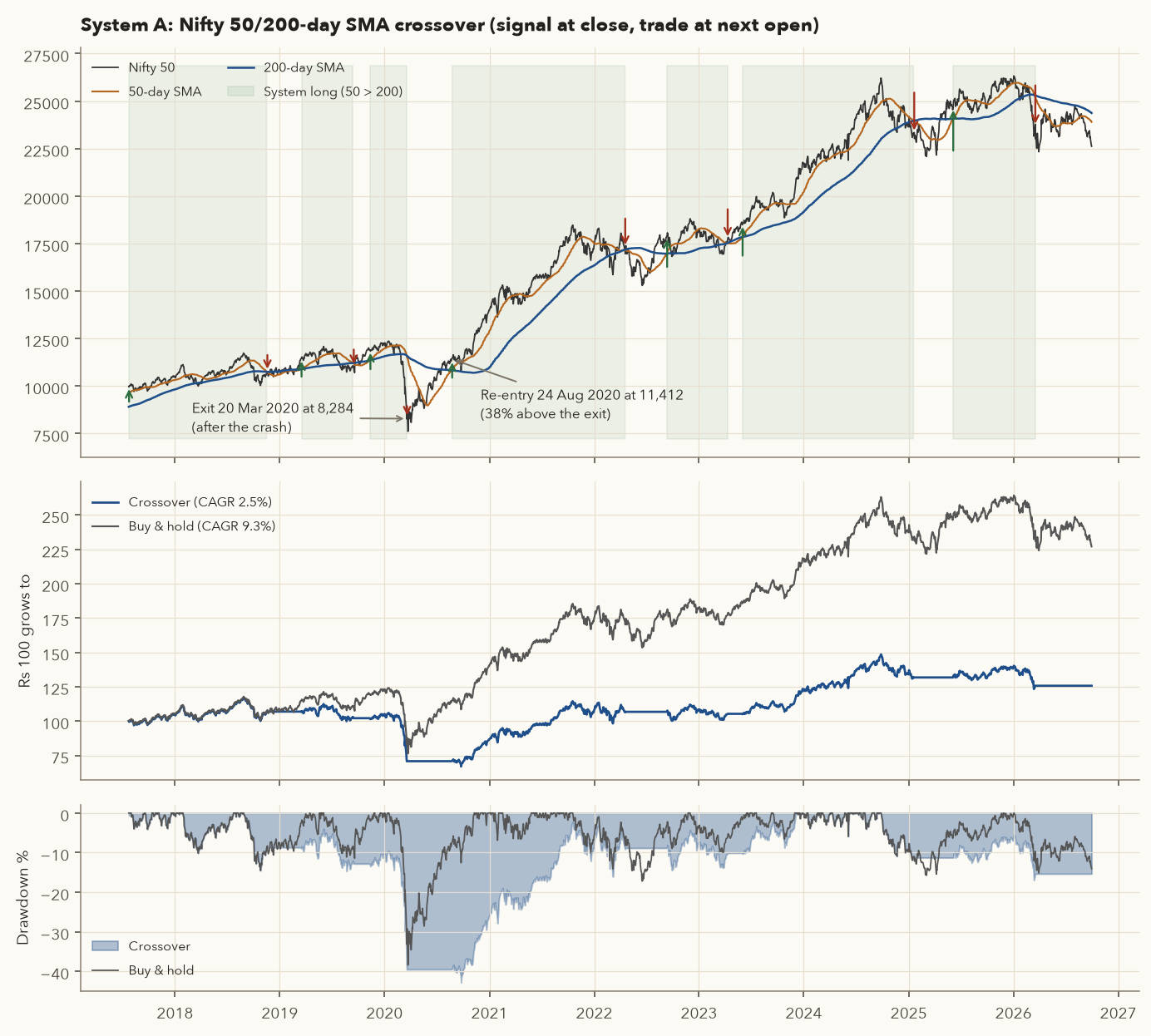
Rules. Universe: Nifty 50 index (in practice a Nifty ETF or futures). Entry: SMA50 closes above SMA200 → buy at the next open. Exit: SMA50 closes below SMA200 → sell at the next open. Size: 100% of capital. Costs: delivery charges (0.1187% buy / 0.1037% sell) + 0.05% slippage per side. Test period: 24 Jul 2017 (first day with a 200-day average in our file) to 30 Sep 2026.
ch12_figures.py.| # | Buy (next open) | Price | Sell (next open) | Price | Return | Days |
|---|---|---|---|---|---|---|
| 1 | 25 Jul 2017 | 10,010.55 | 19 Nov 2018 | 10,731.25 | +7.2% | 482 |
| 2 | 18 Mar 2019 | 11,473.85 | 16 Sep 2019 | 10,994.85 | −4.2% | 182 |
| 3 | 13 Nov 2019 | 11,908.30 | 20 Mar 2020 | 8,284.45 | −30.4% | 128 |
| 4 | 24 Aug 2020 | 11,412.00 | 19 Apr 2022 | 17,258.95 | +51.2% | 603 |
| 5 | 12 Sep 2022 | 17,890.85 | 11 Apr 2023 | 17,704.80 | −1.0% | 211 |
| 6 | 2 Jun 2023 | 18,550.85 | 20 Jan 2025 | 23,290.40 | +25.6% | 598 |
| 7 | 5 Jun 2025 | 24,691.20 | 18 Mar 2026 | 23,632.90 | −4.3% | 286 |
What happened. The system was meant to reduce drawdowns, and in this period it increased them. In the March 2020 COVID crash the averages crossed only on 19 Mar 2020, so the system sold at 8,284, close to the bottom. It bought back on 24 Aug 2020 at 11,412, which is 37.8% higher than the exit. A slow average needs months of falling prices before it turns, so it is late at both ends of a fast V-shaped crash. Over 9.19 years the system turned ₹100 into ₹125.66 (CAGR 2.52%), while buy-and-hold turned it into ₹226.97 (CAGR 9.33%). It was invested 74% of the time. Even if the idle cash had earned 5.5%, CAGR rises only to 3.95%.
| Metric | 50/200 crossover | Nifty buy & hold |
|---|---|---|
| CAGR | 2.52% | 9.33% |
| Volatility | 12.6% | 16.6% |
| Sharpe (rf 5.5%) | −0.17 | 0.30 |
| Sortino | −0.22 | 0.41 |
| Max drawdown | −42.85% (24 Sep 2020) | −38.44% (23 Mar 2020) |
| Calmar | 0.06 | 0.24 |
| Trades / win rate / profit factor | 7 / 42.9% / 2.10 | 1 / – / – |
| Average holding | 356 days | whole period |
| Exposure | 74% | 100% |
A longer test. Over 2009–2026 (17.7 years of Nifty history downloaded separately) the crossover made 4.85% a year against 11.96% for buy-and-hold, with 12 trades and the same −42.85% maximum drawdown. The result does not depend on the start date.
Status today (educational). On 30 Sep 2026 Nifty closed at 22,620.45, the 50-day SMA was 23,901.58 and the 200-day SMA 24,372.85. The system has been in cash since its 18 Mar 2026 exit.
A profit factor of 2.10 sounds great, but with only 7 trades it means almost nothing. The comparison that matters is with the simplest alternative. A rule whose main job is to reduce risk has to be tested on the risk it claims to reduce, and here it failed. For a long-term index investor in this period, staying invested beat timing with the averages. (Varsity's Module 2 introduces moving-average crossovers as a trend-following tool. This test shows why they are better as a filter than as a stand-alone index-timing system.)
7. System B: 55-day breakout on 37 stocks with 1% risk
Hypothesis. Stocks that make a new 55-day high are often in the early part of a long trend: institutions accumulate in stages, and a breakout forces short sellers and sceptics to buy. Most breakouts fail, so we cut failures quickly and let the few big trends run. This is the logic of the 1980s "Turtle" traders' channel-breakout system.
The tool is a Donchian channel: two lines drawn on the chart, the highest high of the last N sessions (upper line) and the lowest low of the last M sessions (lower line). A close above the upper line is a breakout; a close below the lower line ends the trend. With N = 250 (about a year of sessions) the same rule becomes the popular 52-week-high breakout. It trades less often and enters later in a trend. The framework's breakout_52w strategy lets you test that version on the same universe.
Rules.
- Universe: the 37 stocks in the course data set (each trades only after it has enough history).
- Entry: close above the highest high of the previous 55 sessions → buy at the next open + 0.1% slippage.
- Initial stop: signal-day close − 2 × ATR(20) (Wilder). The stop is fixed and does not trail.
- Exit: close below the lowest low of the previous 20 sessions → sell at the next open, or the stop is touched intraday.
- Size: risk 1% of current equity: qty = equity × 1% ÷ (fill − stop); no position above 20% of equity.
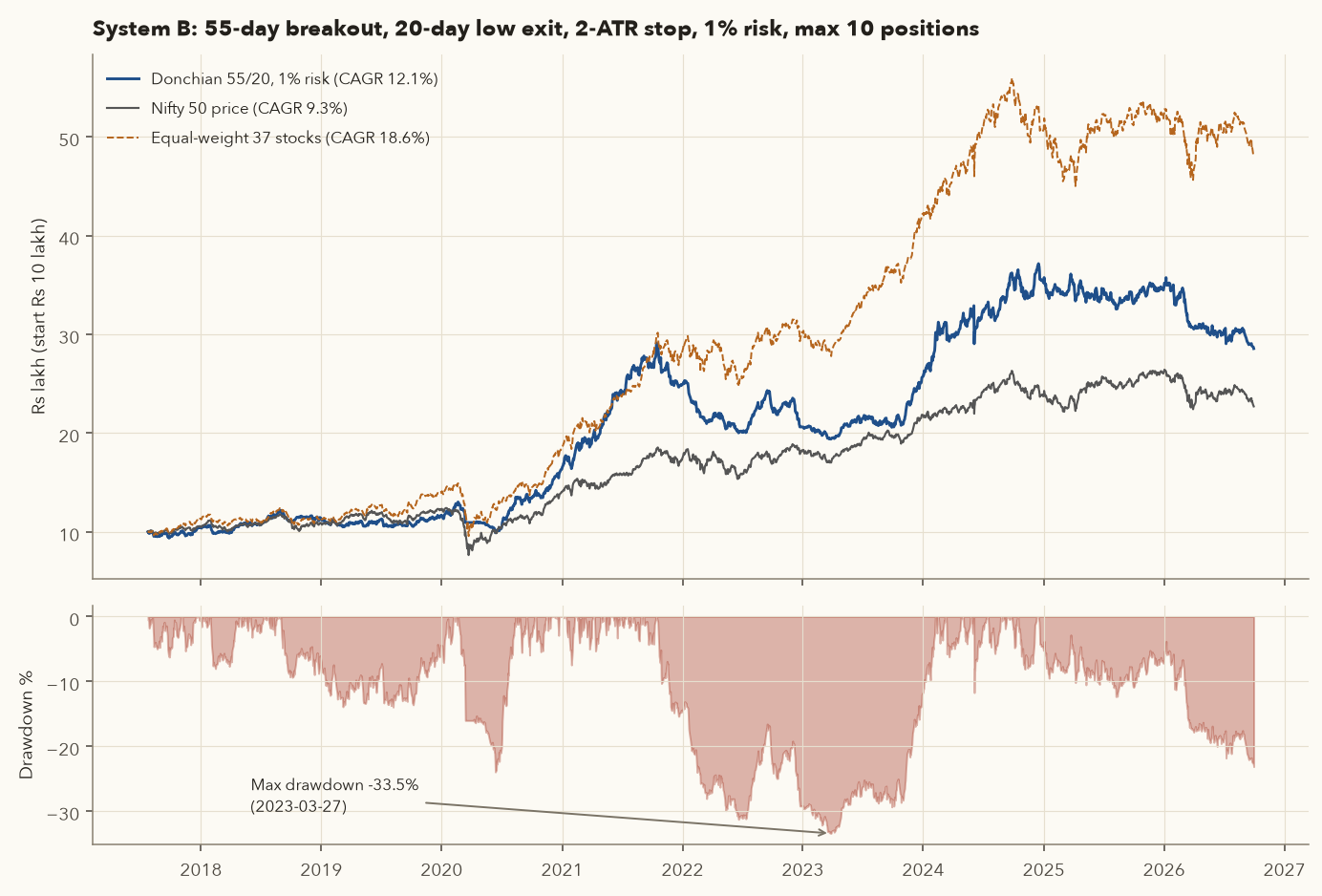
- Portfolio: at most 10 positions; when there are more signals than free slots, take the highest 6-month return first. Capital ₹10 lakh; delivery charges on every leg.
Sizing a breakout with 1% risk (the system's best trade)
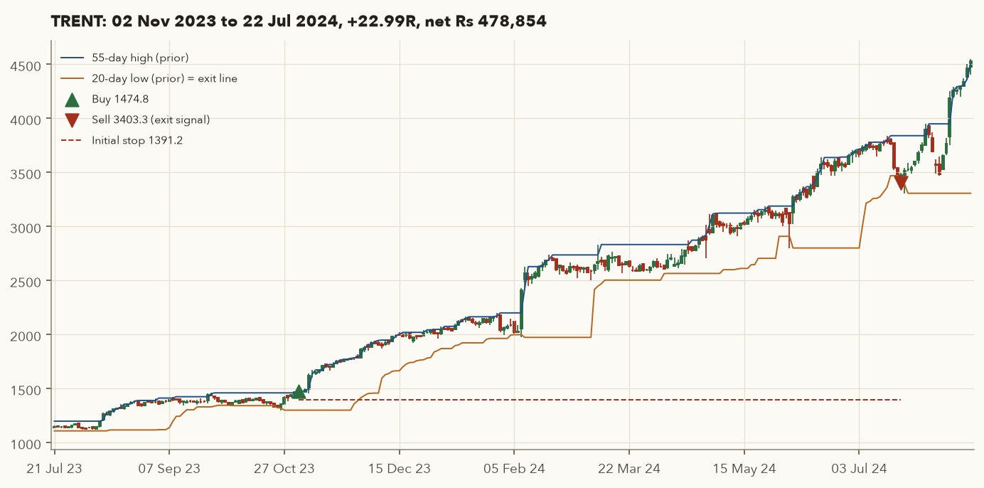
- Signal (1 Nov 2023 close). Close 1,465.10 > previous 55-day high 1,456.67 → breakout. ATR(20) = 36.97, so stop = 1,465.10 − 2 × 36.97 = 1,391.15.
- Equity that evening = ₹20,87,590. Risk budget = 1% = ₹20,876.
- Fill (2 Nov open). 1,473.33 + 0.1% slippage = 1,474.81. Risk per share = 1,474.81 − 1,391.15 = 83.65. Quantity = 20,876 / 83.65 = 249.5 → 249 shares (₹3.67 lakh, 17.6% of equity, under the 20% cap).
- Exit. The stock trended for 8 months. The first close below the 20-day low came on 19 Jul 2024, and the position was sold at the 22 Jul open: 3,403.26 after slippage.
- Result. (3,403.26 − 1,474.81) × 249 − costs ₹1,330 = +₹4,78,854 = +22.99R (R = 83.65 × 249 = ₹20,829).
A typical failed breakout
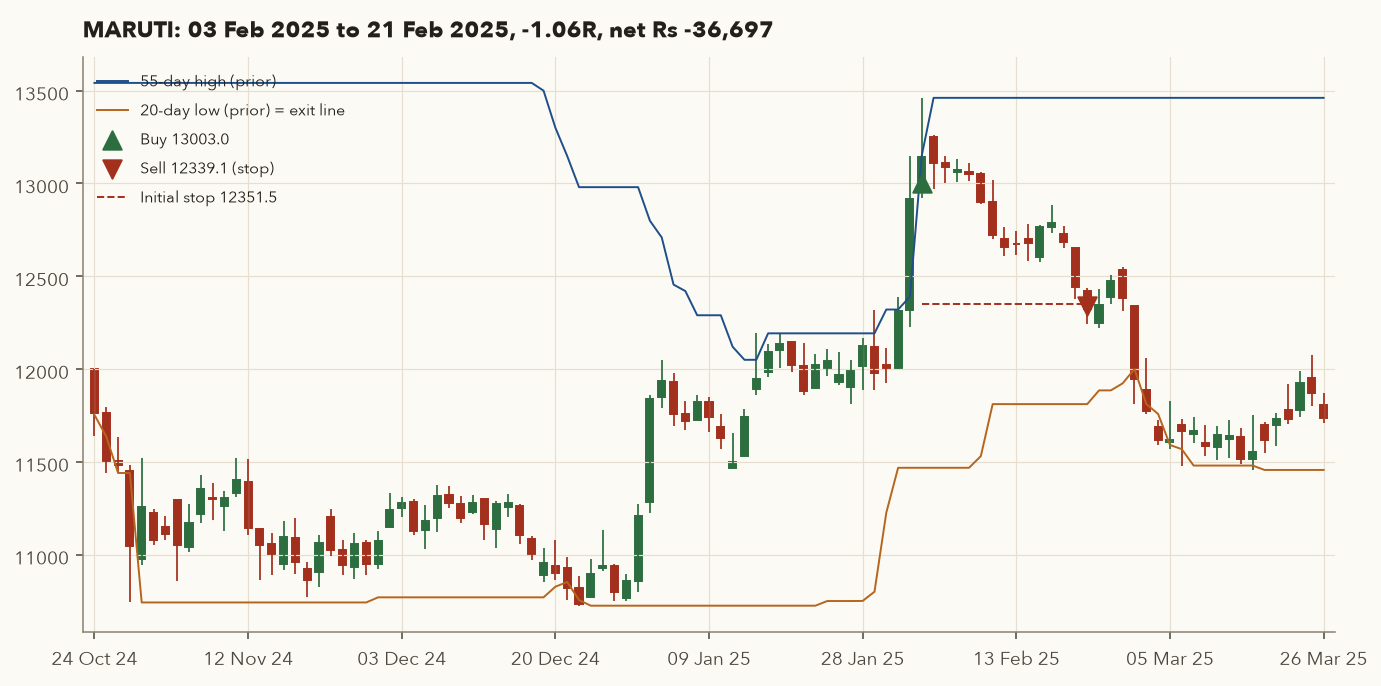
- Signal 1 Feb 2025: close 12,916.50 > 55-day high 12,390. ATR(20) = 282.51 → stop 12,916.50 − 565.02 = 12,351.48.
- Equity ₹34,63,066 → risk ₹34,631. Fill 3 Feb at 12,990 + 0.1% = 13,002.99. Risk/share 651.51 → 53 shares.
- The stock slid back, and the stop was touched on 21 Feb: fill 12,351.48 − 0.1% = 12,339.12.
- P&L = (12,339.12 − 13,002.99) × 53 − ₹1,512 costs = −₹36,697 = −1.06R. A small, planned loss. Seven out of ten trades end like this.
Where the money came from
| Year (exit) | Net P&L (₹) | Year (exit) | Net P&L (₹) |
|---|---|---|---|
| 2017 (Aug–Dec) | −77,125 | 2022 | −1,49,694 |
| 2018 | +1,86,726 | 2023 | −20,222 |
| 2019 | −43,391 | 2024 | +10,38,699 |
| 2020 | +80,235 | 2025 | +2,08,813 |
| 2021 | +10,64,529 | 2026 (to Sep) | −4,33,509 |
- Profits were concentrated. Two years (2021 and 2024) produced more than the entire net profit of ₹18.55 lakh. The 5 best trades (TRENT +₹4.79 L, ADANIENT +₹3.97 L, DIXON +₹2.65 L and two others) produced 84.7% of the total. The best 10% of trades produced 239% of it, so the other 90% lost money as a group. Trend following works this way: you cannot know in advance which trade will be the big one, so you must take them all.
- Long losing streaks are normal. The longest run of consecutive losing trades was 20. Exits: 196 at the stop, 41 by gapping through the stop, 187 on the 20-day-low signal.
- Costs mattered. Without charges and slippage the same rules made 14.06% CAGR (max DD −30.2%). Costs and slippage took about 2 percentage points a year.
(1) Split the test in two and the first half (Jul 2017 – Dec 2021) made 22.8% a year, while the second half (Jan 2022 – Sep 2026) made 1.25% a year, below Nifty's 5.4%. (2) Forty versions with random entries and the same exits and sizing averaged 12.8% CAGR, and 60% of them beat the breakout entry. (3) Adding five once-popular stocks that later collapsed cuts CAGR from 12.1% to 8.3%. Keep these in mind before you trust the 12.1%.
python -m framework.backtest_cli donchian_trend runs the framework's version on the same universe. Its result is close but not identical: CAGR 13.8%, max DD −27.0%, 363 trades, expectancy +0.50R (3 Oct 2017 – 30 Sep 2026). The framework holds at most 8 positions instead of 10, starts trading in October 2017 after a one-year indicator warm-up, uses dividend-adjusted prices and ranks signals by relative strength against Nifty. That two reasonable implementations differ by almost 2 percentage points a year is itself a lesson: small implementation details move results, so never treat a backtest number as precise.
8. System C: RSI(2) mean reversion in an uptrend
Hypothesis. Within a long-term uptrend, sharp 2–3 day sell-offs are often overreactions (forced selling, noise), and prices bounce back within days. So buy short-term weakness in long-term strength. This is the opposite of System B: high win rate, small gains, short holds.
RSI(2) is the ordinary Wilder RSI from Chapter 4, computed over just 2 days instead of 14. With so short a window it swings to extremes after only two down days. A reading below 10 means the last couple of sessions were almost all losses.
Rules. Universe: the same 37 stocks. Trend filter: close > 200-day SMA. Entry: RSI(2) < 10 → buy at the next open + 0.1% slippage. Exit: close > 5-day SMA → sell at the next open; or a time stop after 10 sessions. No price stop (a common design for this style; see the loss example). Size: 10% of equity per position, up to 10 positions; the most oversold signal first. Costs: full delivery charges.
The textbook case, helped by an earnings gap
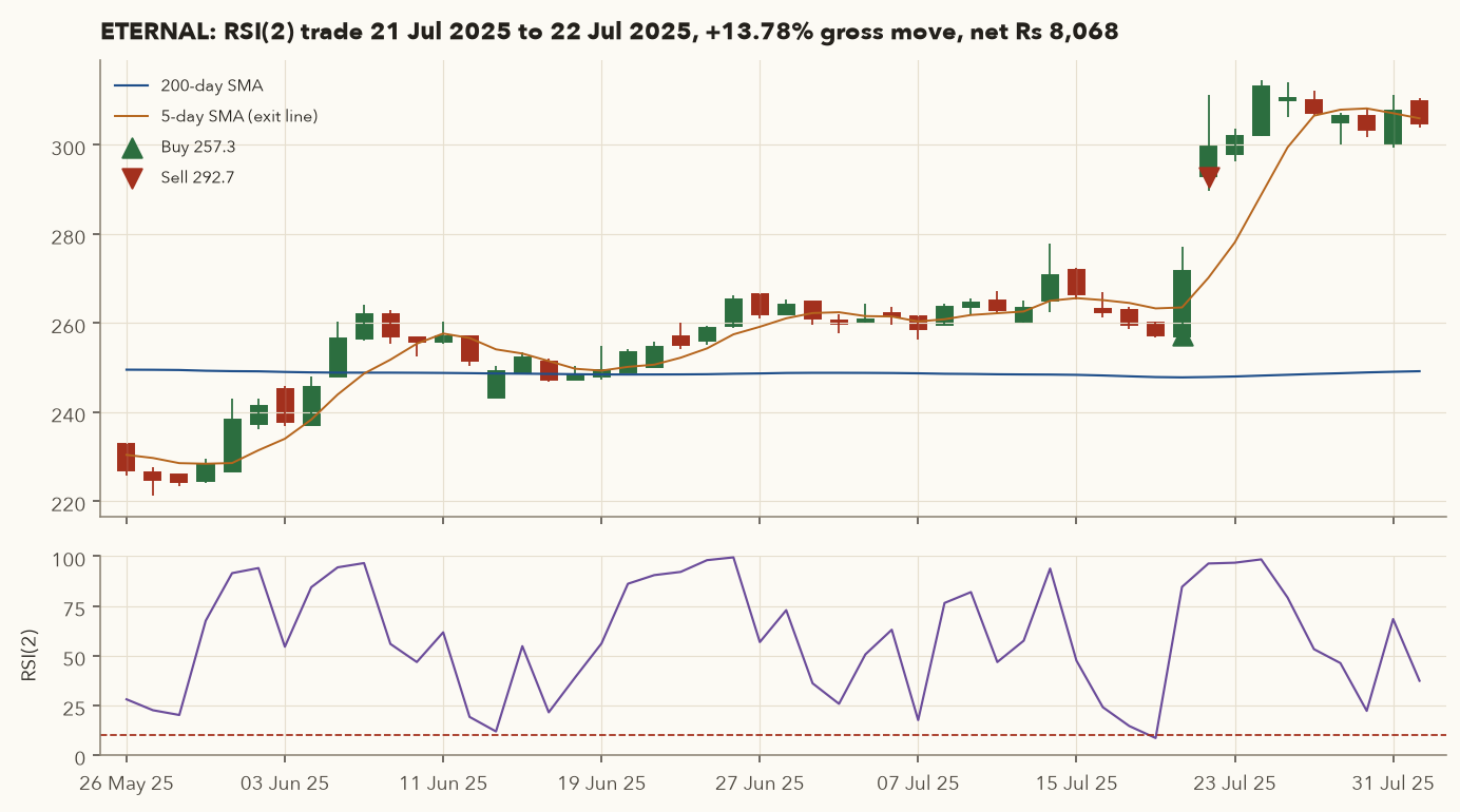
- Signal 18 Jul 2025: close 257.20 > SMA200 247.82 (uptrend), RSI(2) = 8.47 < 10.
- Bought 232 shares on 21 Jul at 257.00 + 0.1% = 257.26. The stock jumped on its quarterly results that day and closed at 271.70, above the 5-day SMA → exit signal.
- Sold 22 Jul at the open, 293.00 − 0.1% = 292.71. Net P&L +₹8,068 (+13.8%, costs ₹157).
- Honest note: most of that gain was the results announcement, not "mean reversion". One lucky trade like this can flatter a small sample.
Why "no stop" plus next-open fills can hurt
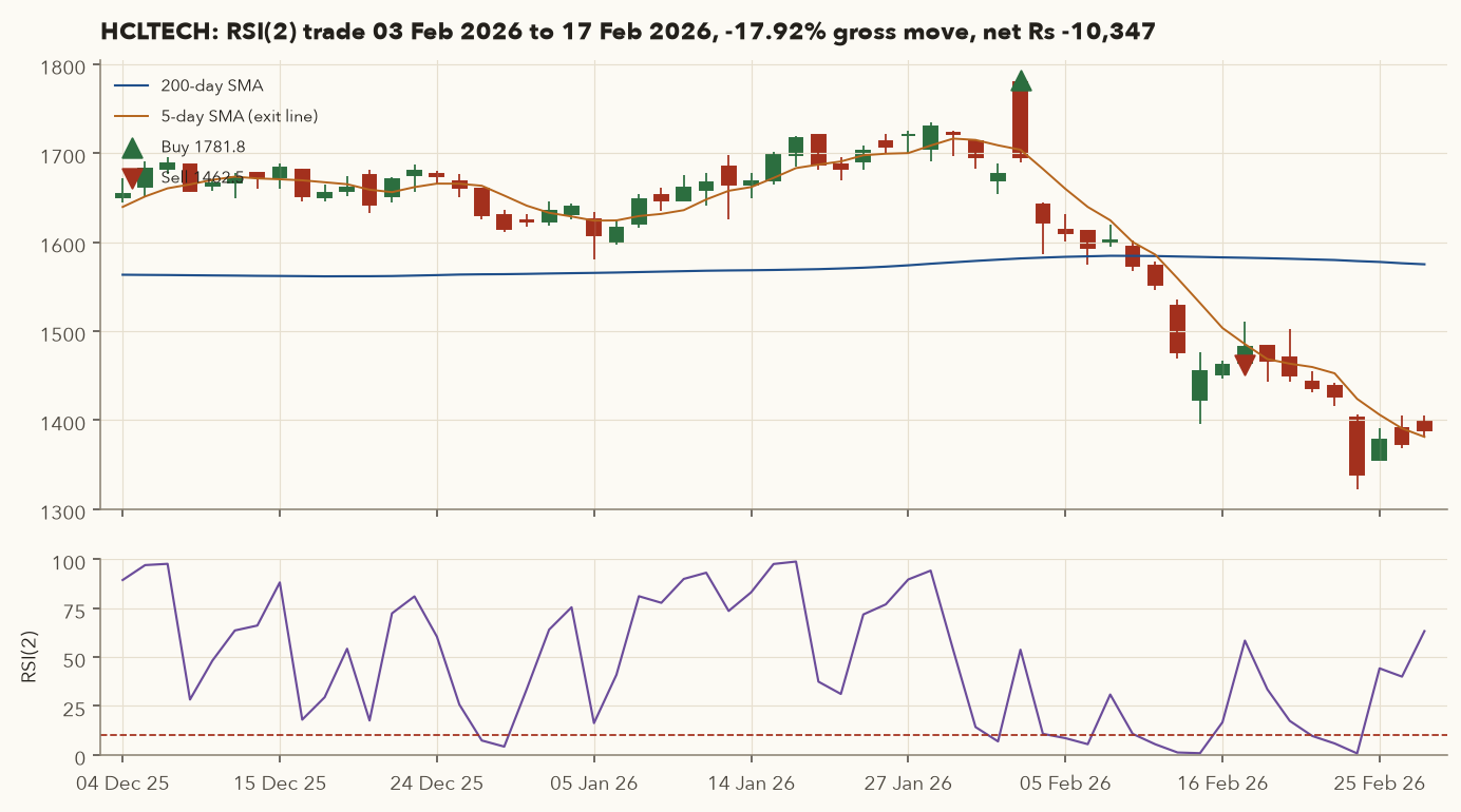
- Signal 2 Feb 2026: close 1,676.80 > SMA200 1,580.32, RSI(2) = 6.89.
- On 3 Feb the whole market gapped up (Nifty opened at 26,308 after a 25,088 close). HCLTECH opened at 1,780, 6.2% above the signal close. The rules still buy: 32 shares at 1,781.78. The "oversold" premise was gone before the order filled.
- IT stocks then sold off hard. The exit condition never triggered, so the 10-session time stop sold on 17 Feb at 1,462.54: −17.9%, −₹10,347.
- Lesson: write rules for gaps ("skip if the open is more than X% above the signal close"). Then test that rule out-of-sample, not on the trade that inspired it.
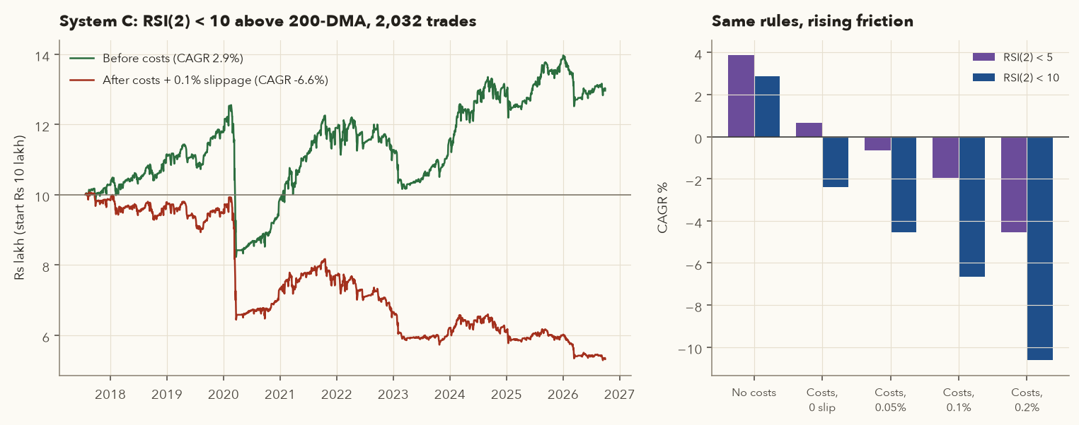
| Version (Jul 2017 – Sep 2026) | Trades | Win rate | Profit factor | Avg trade before charges | CAGR |
|---|---|---|---|---|---|
| RSI(2) < 10, no costs, no slippage | 2,032 | 63.6% | 1.11 | +0.17% | +2.87% |
| RSI(2) < 10, delivery costs, 0 slippage | 2,032 | 59.1% | 0.91 | +0.17% | −2.41% |
| RSI(2) < 10, costs + 0.1% slippage (base case) | 2,032 | 55.5% | 0.77 | −0.03% | −6.64% |
| RSI(2) < 5, no costs | 1,221 | 65.0% | 1.25 | +0.32% | +3.87% |
| RSI(2) < 5, costs + 0.05% slippage | 1,221 | 58.9% | 0.96 | +0.21% | −0.64% |
Diagnosis. The edge is real but tiny. The average trade earned +0.17% before costs, while a round trip of delivery charges on a ~₹1 lakh position costs about 0.24% (0.2225% plus the ₹15.34 DP charge), before any slippage. After costs and 0.1% slippage, ₹10 lakh shrank to ₹5.32 lakh (−6.6% a year, max DD −47.5%), and ₹3.64 lakh went in costs. Charges alone, with zero slippage, already turned the result negative (−2.41%). A 63.6% win rate made it feel like a good system the whole time.
High-turnover, small-edge systems are the most sensitive to costs. Delivery trades in India pay 0.1% STT on both sides. Before building a short-holding system, estimate its average gross trade, and if it is not comfortably above ~0.5%, stop there. (Many RSI(2) results published for US markets assume near-zero costs; Indian delivery costs are different.)
9. The three systems side by side
| Metric | A: 50/200 on Nifty | B: 55-day breakout | C: RSI(2) | Nifty buy & hold |
|---|---|---|---|---|
| Period | Jul 2017 – Sep 2026 | Jul 2017 – Sep 2026 | Jul 2017 – Sep 2026 | Jul 2017 – Sep 2026 |
| CAGR | 2.52% | 12.10% | −6.64% | 9.33% |
| Volatility | 12.6% | 15.7% | 11.4% | 16.6% |
| Sharpe | −0.17 | 0.47 | −1.04 | 0.30 |
| Sortino | −0.22 | 0.64 | −1.27 | 0.41 |
| Max drawdown | −42.9% | −33.5% | −47.5% | −38.4% |
| Calmar | 0.06 | 0.36 | −0.14 | 0.24 |
| Trades | 7 | 424 | 2,032 | – |
| Win rate | 42.9% | 30.4% | 55.5% | – |
| Profit factor | 2.10 | 1.53 | 0.77 | – |
| Avg holding | 356 days | 55 days | 6 days | – |
| Exposure (days with a position) | 74% | 99% | 84% (avg 36% invested) | 100% |
Notice three things. The system with the lowest win rate (B) was the only one that made money. The system with the best profit factor (A) had too few trades for that number to mean anything. And B beat Nifty while holding 37 hand-picked stocks; Section 10.2 shows how much of that is the hand-picking.
10. Backtesting pitfalls, each demonstrated on real data
A backtest can only be wrong in one direction that matters: it can make a bad system look good. Each of the following mistakes makes results look better than reality, and each is shown below on our data.
10.1 Look-ahead bias: using tomorrow's information today
Look-ahead means a decision in the backtest uses information that was not available yet. The commonest version is one missing .shift(1). Take a simple rule, "be long Nifty when it closes above its 20-day SMA", and code it three ways.
sig = (close > close.rolling(20).mean()).astype(int)
ret = close.pct_change()

buggy   = (1 + sig * ret).cumprod()            # WRONG: today's close decides today's return
shifted = (1 + sig.shift(1) * ret).cumprod()   # assumes a fill at the signal day's close, no costs
correct = vector_backtest(df, sig, costs)      # fill at next open, pay costs (Section 4)
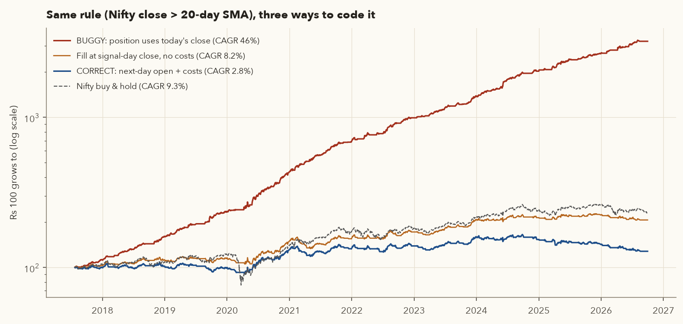
| Implementation | CAGR | Sharpe | Max DD |
|---|---|---|---|
| Buggy (no shift) | 45.8% | 3.41 | −6.7% |
| Fill at signal-day close, no costs | 8.2% | 0.31 | −16.2% |
| Correct: next open + costs + slippage | 2.75% | −0.22 | −22.7% |
Why the bug is so profitable. If today's close is above the 20-day average, today was probably an up day. The buggy code "knew" the day would be up and was long for it. The result is a ₹100 → ₹3,193 equity curve, a Sharpe ratio of 3.4 and a maximum drawdown of only 6.7%. If a simple rule shows a Sharpe ratio above 2 and an almost straight equity curve, assume a bug first. The honest version made 2.75% a year after its 115 round trips, which is below buy-and-hold.
Other ways look-ahead sneaks in: computing the mean and SD of a ratio over the whole period and then trading inside that period (Varsity's Method 1 example does this; see Section 11), using today's high to set today's entry, using quarterly results before their announcement date, and using index membership as of today.
10.2 Survivorship bias: our universe is today's winners
The 37 stocks in this course were chosen in 2026, as today's large, well-known names. Many are there because they did well (TRENT, BEL, HAL, DIXON, ADANIENT). A trader in July 2017 could not have known that list. Popular names in 2017 included YES Bank, Zee Entertainment, Indiabulls Housing Finance (now Sammaan Capital), Vodafone Idea and IndusInd Bank. We downloaded their history and added them back.
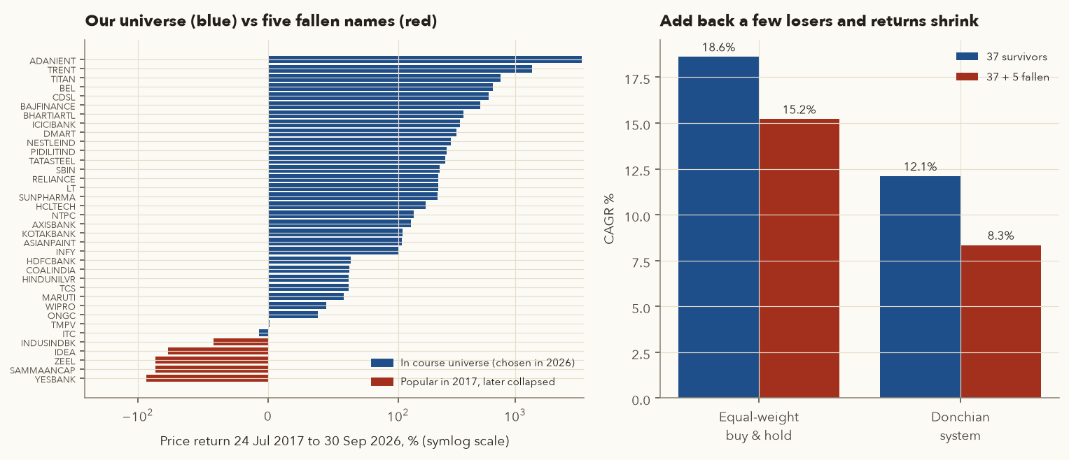
- Price returns of the five: YESBANK −93.4%, SAMMAANCAP −86.8%, ZEEL −86.5%, IDEA −76.6%, INDUSINDBK −42.0%. Of the 31 course stocks listed by July 2017, the median return was +218%, and only ITC was slightly negative on price (its 2025 hotels demerger and large dividends are not in a price-only return).
- Equal-weight buy-and-hold: 18.6% CAGR with 37 survivors → 15.2% with the five added.
- System B: 12.1% → 8.3% CAGR, now below Nifty's 9.3%. The breakout system lost ₹1.00 L on INDUSINDBK, ₹0.60 L on YESBANK, ₹0.46 L on SAMMAANCAP, ₹0.41 L on ZEEL and ₹0.05 L on IDEA.
Even five names, out of the dozens that left the Nifty since 2017, wipe out the system's edge. The proper fix is a point-in-time universe: on each test date, use only the stocks that were in the index (or met your liquidity rules) on that date, including ones that were later delisted. NSE publishes historical index changes. Until you have that data, treat any stock-picking backtest on a modern list as an upper bound.
10.3 Overfitting: the best parameters of the past
Overfitting means tuning rules until they match past noise. We tested 100 fast/slow SMA combinations on Nifty (fast 10–100, slow 50–300), choosing parameters on 2009–2017 (in-sample) and then checking them on 2018–Sep 2026 (out-of-sample), with costs.
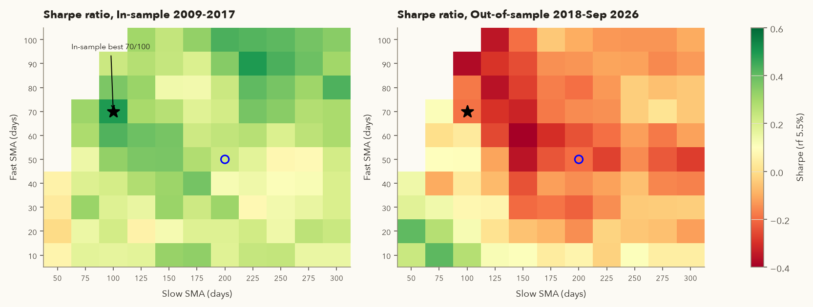
- The in-sample winner, 70/100, had Sharpe 0.49 and CAGR 11.96% in 2009–2017. Out-of-sample: Sharpe −0.19, CAGR 2.46%, rank 76 of 100.
- The out-of-sample winner (10/75) had ranked 76th in-sample. Across all 100 pairs, the correlation between in-sample and out-of-sample Sharpe was −0.32: being good in the past was, if anything, a bad sign. The top 10 in-sample pairs had a median out-of-sample rank of 52.5, no better than random.
- None of the 100 pairs beat buy-and-hold in-sample (14.8%), and only 2 did out-of-sample (9.25%).
What the heatmap shows: a robust idea gives a broad plateau of decent results. A fragile one gives isolated bright spots that move around from period to period. Here the in-sample "best" was a bright spot.
10.4 Out-of-sample splits and walk-forward testing
Two habits protect you. (1) Hold out data. Develop on one period, then test once on a period you never looked at. System B's halves (fixed rules, nothing re-tuned) are a sobering example:
| Period | System B CAGR | Max DD | Trades | Expectancy | Nifty CAGR |
|---|---|---|---|---|---|
| 24 Jul 2017 – 31 Dec 2021 | 22.8% | −24.0% | 204 | +0.47R | 13.3% |
| 1 Jan 2022 – 30 Sep 2026 | 1.25% | −24.6% | 237 | +0.06R | 5.4% |
(2) Walk forward. If you insist on optimising, do it the way you would have to live: each January, pick the best SMA pair using only the previous 3 years, trade it for the next 12 months, and repeat.
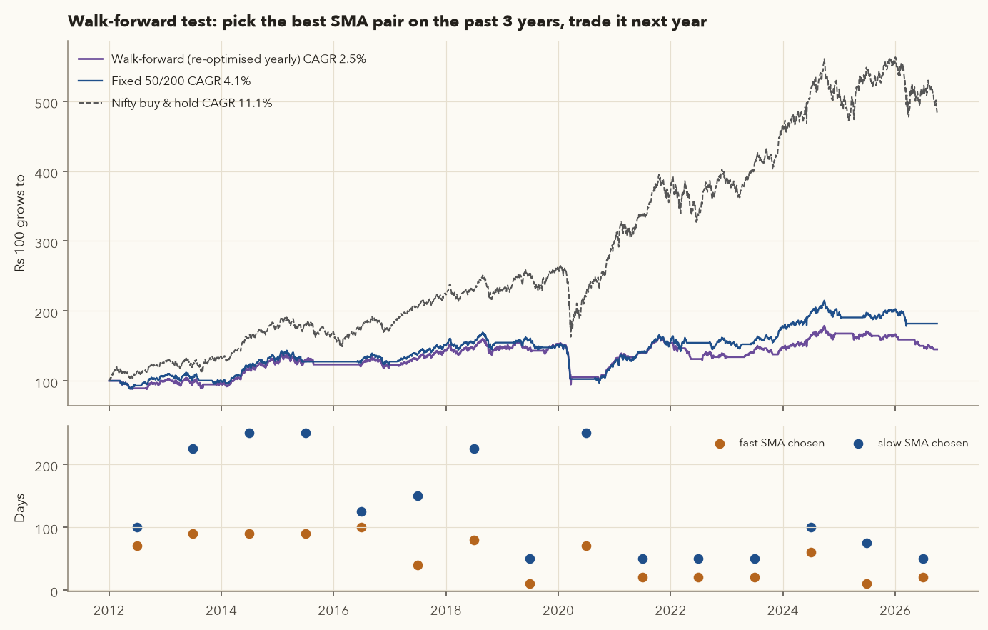
Result: walk-forward 2.55% CAGR vs fixed 50/200 4.14% vs buy-and-hold 11.14% (Jan 2012 – Sep 2026). Re-optimising made things worse. The "best" parameters kept changing, a sign that there was no stable edge to find.
10.5 Transaction costs and slippage
Seen already: System B lost about 2 points of CAGR to friction (14.1% → 12.1%). System C went from +2.9% to −6.6%. A good habit is to double your slippage assumption and check that the system still works. If doubling slippage kills it, the edge is too thin to trade. For futures, remember STT is now 0.05% on the sell side, and an index-futures position that you hold for a year pays two extra legs of charges at every monthly roll (sell the expiring contract, buy the next one), on top of the original buy and the final sell.
10.6 Small samples: luck looks like skill
How many trades do you need? We resampled System B's 424 trade results (in R) 10,000 times.
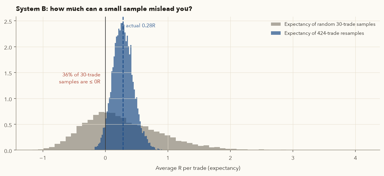
- The system's real first 30 trades averaged −0.51R. A trader judging it on those would have quit.
- 36.5% of random 30-trade samples have zero or negative expectancy, even though the system's overall expectancy is +0.28R. The 90% range for a 30-trade sample is −0.58R to +1.39R.
- Even with all 424 trades, the 95% confidence interval for expectancy is −0.02R to +0.63R. It still includes zero. Nine years of data are not enough to prove this edge statistically.
- Shuffling the order of the same 424 trades 5,000 times gives a median worst drawdown of −35.8R (5% of orderings: worse than −56.8R). At 1% of current equity risked per trade, −35.8R compounds to about −30% of equity (\(0.99^{35.8} - 1\)) and −56.8R to about −43%. Open trades swing further before they close, so real equity drawdowns are deeper than these closed-trade figures. Plan for 35–45%, even though the backtest's single history showed −33%.
10.7 A null model: is the entry rule doing the work?
Replace the breakout entry with a coin flip (each stock has a 2% chance of a "signal" each day). Keep the same universe, stops, 20-day-low exits, 1% sizing and costs, and run it 40 times with different random seeds.
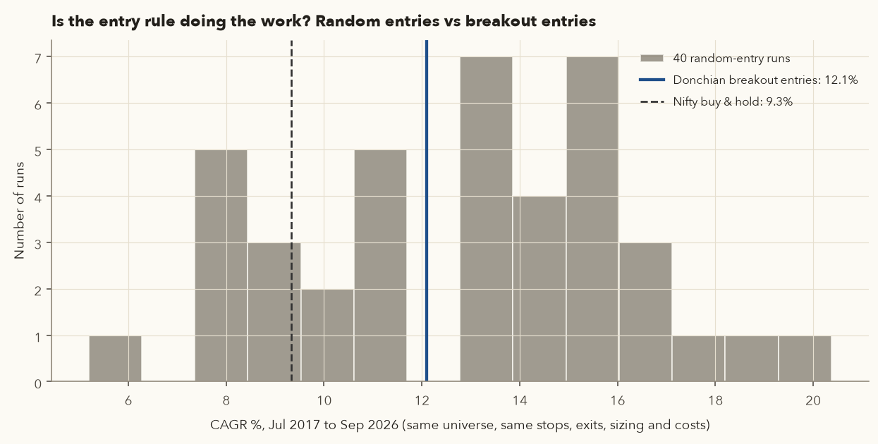
The random-entry runs averaged 12.8% CAGR (median 13.4%, range 5.2% to 20.4%), and 60% of them beat the breakout version. So System B's results come from the exits and sizing (cut losers, let winners trend) applied to a universe that went up, not from clever entries. That is useful to know: it tells you where to spend your research time.
10.8 Other traps worth a checklist line
- Bad data. Missed splits, bonuses and demergers create fake 50% "crashes". The course framework had to fix TRENT, CDSL and Tata Motors' 2025 demerger by hand. Holiday filler bars (zero volume, flat price) distort ATR. Always plot your data and scan for gaps over 20%.
- Dividends. A price-only backtest understates buy-and-hold returns by roughly the dividend yield (about 1–1.5% a year for Nifty).
- Liquidity and capacity. A fill at the open is realistic for ₹5 lakh in HDFC Bank, not for ₹5 crore in a small cap.
- Regime change. System B's two halves show that one decade can contain two very different markets.
- Taxes. Short holding periods mean 20% STCG instead of 12.5% LTCG above ₹1.25 lakh (Chapter 13). A pre-tax backtest flatters active systems against buy-and-hold.
11. Pair trading, Method 1: ratio and density curve
11.1 The logic: two roads that run side by side
Varsity explains pair trading with a picture. Think of a highway and the service road next to it. They climb, dip and cross rivers together. At one spot the service road bends around a tree, then comes back alongside the highway. Two businesses that are truly alike, such as two large private banks with the same products, customers and regulator, are like those roads. Industry-wide news (an RBI rate move, a credit cycle) moves both. A local event (one bank's results, a senior executive leaving, a burst of speculation) can push one away from the other for a while. That is the tree. If the relationship holds, the gap should close, and you profit by buying the relatively cheap stock and selling the relatively expensive one.
Varsity stresses this point: being long one stock and short another is relative value or statistical arbitrage, not a market-neutral position. The two stocks can and do move differently, and that difference is exactly your risk. Pair trades need short positions held overnight, which in India means stock futures, with their lot sizes, margins and expiries (Chapter 9). Only stocks in the F&O segment can be paired this way.
11.2 The vocabulary (Varsity PTM1, chapters 1–2)
- Spread: difference between the two stocks' daily % changes. Mainly useful intraday.
- Differential: difference between the two closing prices.
- Ratio: price of stock A ÷ price of stock B. The variable Method 1 tracks, end of day.
- Divergence / convergence: expecting the ratio to move away from / back towards its average.
- Correlation: between −1 and +1, how closely the two move together. Varsity uses a correlation of daily returns of roughly 0.75 or more to qualify a pair. Correlation tells you direction, not size: two stocks with correlation 0.8 can still drift apart for months.
11.3 The density curve
Treat the ratio's history as roughly normal with mean \(\mu\) and SD \(\sigma\). Varsity uses Excel's NORM.DIST(ratio, mean, SD, TRUE), which is the cumulative normal probability:
- \(\text{ratio}_t\)
- Today's closing price of stock A divided by today's closing price of stock B.
- \(\mu\)
- The average ("mean") of the ratio over the look-back window (Varsity uses the whole history in the sheet).
- \(\sigma\)
- The standard deviation (SD) of the ratio over the same window: how far it typically strays from its mean.
- \(\frac{\text{ratio}_t - \mu}{\sigma}\)
- The z-score: how many SDs today's ratio is above (positive) or below (negative) its mean.
- \(\Phi\)
- The cumulative normal function (Excel's
NORM.DIST(…, TRUE)). It turns a z-score into a number between 0 and 1: the share of a normal bell curve that lies below that z-score. - \(D_t\)
- The density value, between 0 and 1. 0.5 means the ratio is at its mean.
How it works: subtract the mean from today's ratio, divide by the SD to get the z-score, then feed it to \(\Phi\). Read the result like this: \(D\) = 0.16 ≈ −1 SD, 0.025 ≈ −2 SD, 0.003 ≈ −2.75 SD; 0.84 ≈ +1 SD, 0.975 ≈ +2 SD, 0.997 ≈ +2.75 SD. Varsity calls 0.003 and 0.997 the "3 SD" levels, borrowing the rule that 99.7% of a normal curve lies within ±3 SD. That 99.7% is split between both tails, though, so each tail beyond ±3 SD holds only 0.13% (\(\Phi(-3) = 0.0013\)). We keep Varsity's 0.003 and 0.997 levels, but call them what they are: about ±2.75 SD. A value near 0 means A is unusually cheap against B; near 1, unusually expensive. The ICICI/HDFC example below works it through.
| Trade | Trigger (density) | Meaning | Exit | Stop |
|---|---|---|---|---|
| Long the ratio (buy A, sell B) | between 0.025 and 0.003 | ratio about 2 to 2.75 SD below its mean | as it moves back towards the mean (Varsity's example closed near 0.25) | 0.003 or lower (about −2.75 SD or further) |
| Short the ratio (sell A, buy B) | between 0.975 and 0.997 | ratio about 2 to 2.75 SD above its mean | back below 0.975 or nearer the mean | 0.997 or higher (about +2.75 SD or further) |
Varsity also asks for rupee neutrality: roughly equal rupee value on each side, so you are betting on the ratio, not on the market. Method 1 comes from Mark Whistler's book Trading Pairs. Varsity presents it as the simpler foundation before Method 2.
Method 1 on the classic Indian pair
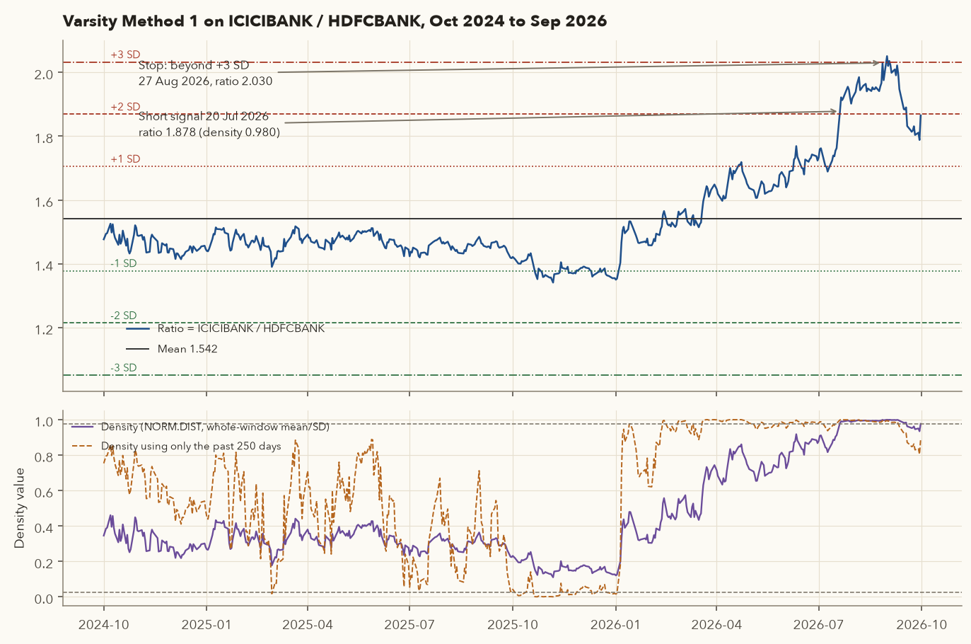
- Qualify the pair. Over 494 sessions (1 Oct 2024 – 30 Sep 2026), the correlation of daily returns was 0.515, well below Varsity's ~0.75 guideline. (Correlation of price levels was 0.423; use returns, because price levels of any two trending stocks look correlated.) Varsity calls the correlation number "sacred" and wants it above 0.75, though it relaxed this for its own Axis/ICICI example. Treat 0.515 as a warning.
- Pair stats. Mean ratio 1.5416, median 1.4772, SD 0.16358. Bands: −3 SD 1.0509, −2 SD 1.2144, −1 SD 1.3780, +1 SD 1.7052, +2 SD 1.8688, +3 SD 2.0323. Mean above median warns that the distribution is skewed, not normal.
- Signal. On 20 Jul 2026 the ratio was 1,460.20 / 777.60 = 1.8778. \(z = (1.8778 - 1.5416)/0.16358 = 2.055\), \(D = \Phi(2.055) = 0.980\), inside 0.975–0.997 → short the ratio: sell ICICI, buy HDFC.
- Trade (₹5 lakh per leg at the next open, 21 Jul): short 340.1 ICICI at 1,470.00, long 650.1 HDFC at 769.15.
- Stop. The ratio kept rising. On 27 Aug 2026 it hit 2.0295 (z = 2.98, density 0.9986, past the 0.997 stop). Exit at the 28 Aug open: ICICI 1,435.00, HDFC 710.85. ICICI short made +₹11,905, HDFC long lost −₹37,899: net −₹25,994 before costs. The ratio peaked at 2.0508 on 31 Aug.
Why it failed, and a hidden look-ahead. The ratio did not swing around a stable mean. It trended: it averaged 1.462 in Oct–Dec 2024 and 1.892 in Jul–Sep 2026, because HDFC Bank fell well behind ICICI. The relationship changed, which is the main risk in any pair trade. There is a second problem. The mean and SD came from the whole two-year window, including the months after the signal. Using only the 250 days before each date (the dashed line in the lower panel), the density on 20 Jul 2026 was already 0.998, beyond the stop level, so an honest trader would never have entered. Method 1 as usually shown in spreadsheets has look-ahead built in. Always compute the statistics on a rolling past window.
12. Pair trading, Method 2: regression, error ratio, ADF, z-score
Varsity's second method (its author's own improvement) asks a sharper question: not "do these move together?", but "is there a stable linear relationship whose errors keep snapping back?"
12.1 Straight line and linear regression
- \(t\)
- A trading day in the window (the last 200 sessions).
- \(y_t\)
- The closing price of the dependent stock (the "Y" stock) on day \(t\), in ₹.
- \(x_t\)
- The closing price of the independent stock (the "X" stock) on the same day, in ₹.
- \(\beta\)
- The slope ("beta"): how many rupees \(y\) tends to move for a ₹1 move in \(x\). It is also the hedge ratio: \(\beta\) shares of X against each share of Y.
- \(c\)
- The intercept, in ₹: the part of \(y\)'s price the line does not explain through \(x\).
- \(\varepsilon_t\)
- The residual ("epsilon"), in ₹: actual \(y_t\) minus the predicted \(\beta x_t + c\). Positive means Y is above where the line says it should be.
How it works: plot the 200 pairs of closes as dots and draw the straight line that fits them best. "Best" means least squares: the line that makes the sum of the squared residuals as small as possible (Excel's regression tool or SLOPE/INTERCEPT does this). The line gives \(\beta\) and \(c\); each day's gap from the line is that day's residual.
Example (TCS on INFY, Section 12.3): TCS = 1.8235 × INFY + 211.31. On 30 Sep 2026 INFY closed at 994.10, so the line predicts 1.8235 × 994.10 + 211.31 = 2,024.05. TCS actually closed at 2,050.60, a residual of +26.55.
From a trader's view, Varsity reads each term like this. \(\beta x\) is hedged: hold 1 share of y against \(\beta\) shares of x. \(c\) is not hedged, so we want it small relative to the price. \(\varepsilon\) is what we trade: if it is stationary (mean-reverting), its extremes are opportunities.
12.2 The error ratio: which stock is Y?
Regress both ways and compare. Varsity's "error ratio" (its own term, not a standard statistic):
- SE of the intercept
- The standard error of \(c\), in ₹: how uncertain the estimate of the intercept is. A regression output (Excel's
LINESTor Data Analysis tool) prints it next to the intercept. - SE of the regression
- The typical size of the residuals, in ₹: roughly their standard deviation. Excel labels it "Standard Error" in the regression statistics.
How it works: run the regression twice, once with each stock as Y. For each run, divide the intercept's SE by the regression's SE. Both are in rupees, so the ratio has no units. Pick the direction with the lower error ratio: the intercept (the part you cannot hedge) is estimated more precisely there.
Error ratio both ways
| Direction | Slope β | Intercept | SE intercept | SE regression | Error ratio |
|---|---|---|---|---|---|
| Y = HDFCBANK, X = ICICIBANK | 0.2048 | 541.11 | 130.70 | 90.16 | 130.70 / 90.16 = 1.4497 |
| Y = ICICIBANK, X = HDFCBANK | 0.1088 | 1,265.01 | 42.17 | 65.71 | 42.17 / 65.71 = 0.6418 |
So Y = ICICI, X = HDFC. But look at the fit: R² = 0.022. HDFC's price explains about 2% of ICICI's price movement in this window, and the intercept (1,265) is 95.7% of ICICI's price. The "hedge" hedges almost nothing. The ADF test (next) agrees: p = 0.59. In 2026 these two banks were not a pair in the statistical sense, whatever their businesses look like.
Do the algebra and the Y prices cancel out. The standard error of the intercept is the regression's standard error times \(\sqrt{1/n + \bar x^2/\sum (x-\bar x)^2}\), so
\[ \text{Error ratio} = \sqrt{\frac1n + \frac{\bar x^{\,2}}{\sum (x_t-\bar x)^2}} = \frac{1}{\sqrt n}\sqrt{1 + \frac{1}{\text{CV}_x^{\,2}}},\qquad \text{CV}_x = \frac{\text{SD of }x}{\text{mean of }x} \]It depends only on the X stock. It picks as X whichever stock's price varied more relative to its own level over the window. In this window ICICI's price varied by only 4.9% of its mean (CV 0.049, error ratio 1.4497), while HDFC's varied by 11.1% (CV 0.111, error ratio 0.6418). That is why TCS/INFY and WIPRO/INFY in the pair sheet below both show exactly 0.4388: it is INFY's number. The error ratio is a reasonable tie-breaker for choosing Y and X. It says nothing about whether the pair is any good. R² and, above all, the ADF test do that job.
12.3 Stationarity and the ADF test
Varsity's check: the residuals must be stationary. That means (1) a stable mean, (2) a stable SD, and (3) little autocorrelation. If they are, the two stocks are cointegrated. The Augmented Dickey-Fuller (ADF) test formalises it. Regress the change in the residual on its previous level:
- \(\varepsilon_t\)
- The residual from the pair equation on day \(t\), in ₹. \(\varepsilon_{t-1}\) is yesterday's residual.
- \(\Delta\)
- "Change in" ("delta"). \(\Delta\varepsilon_t = \varepsilon_t - \varepsilon_{t-1}\): how much the residual moved today. \(\Delta\varepsilon_{t-1}\) is yesterday's move (the "1 lag").
- \(a\)
- A constant fitted by the regression.
- \(\gamma\)
- ("gamma") How today's change depends on yesterday's level. Negative means a high residual tends to fall and a low one to rise.
- \(b\)
- How today's change depends on yesterday's change. It soaks up short-term momentum so it does not distort \(\gamma\).
- \(u_t\)
- What is left unexplained on day \(t\) (noise).
- \(\hat\gamma,\ \text{SE}(\hat\gamma)\)
- The hat means "estimated from the data". \(\hat\gamma\) is the fitted value of \(\gamma\); \(\text{SE}(\hat\gamma)\) is its standard error, how uncertain that estimate is.
- \(t_{\text{ADF}}\)
- The ADF t-statistic: the estimate divided by its uncertainty. No units.
- From the 200 residuals, build three columns: today's change, yesterday's level and yesterday's change.
- Regress today's change on the other two. This gives \(\hat\gamma\) and its SE.
- Divide to get \(t_{\text{ADF}}\). If \(\gamma\) is clearly negative, a big residual tends to be followed by a move back: mean reversion. A more negative t-statistic is stronger evidence.
- Turn the t-statistic into a p-value (the table below gives the critical values). Varsity accepts a pair if the ADF p-value is below 0.05. The TCS/INFY example below has t = −2.90 and fails.
We coded the ADF test in plain numpy (no statsmodels), and found the p-value by simulation. One detail matters a lot. When the residuals come from a regression you just fitted, the regression has already made them look as stationary as possible. So the usual Dickey-Fuller critical values are too lenient. We simulated 4,000 pairs of independent random walks (n = 200), regressed one on the other, and recorded the ADF t-statistic of the residuals. This is the Engle-Granger approach.
| Critical value (n = 200) | 1% | 5% | 10% |
|---|---|---|---|
| Plain series (Dickey-Fuller) | −3.51 | −2.86 | −2.54 |
| Regression residuals (Engle-Granger, used here) | −3.79 | −3.31 | −3.03 |
A pair needs an ADF t-stat below about −3.3 to pass at 5%. Using −2.86 would accept many pairs that are just two random walks that happened to wander together.
A beautiful fit that still fails the test
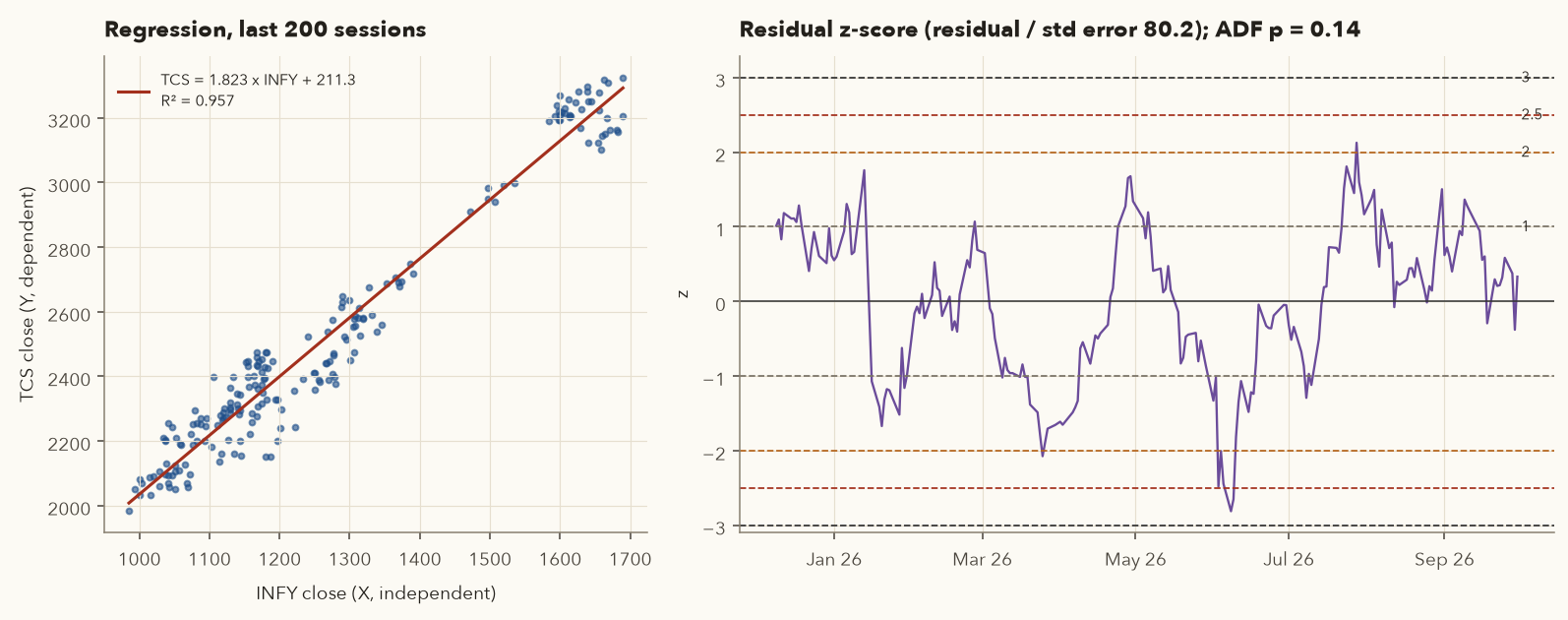
- Error ratio. TCS on INFY: 35.18 / 80.16 = 0.4388. INFY on TCS: 0.4678. So Y = TCS.
- Equation. TCS = 1.8235 × INFY + 211.31, R² = 0.957 (both fell sharply together in 2026).
- Today's residual. 30 Sep 2026: predicted TCS = 1.8235 × 994.10 + 211.31 = 2,024.05; actual 2,050.60; residual +26.55; z = 26.55 / 80.16 = +0.33. No signal.
- Stationarity by eye. Residual means over the three thirds of the window: +10.3, −48.0, +38.3 (TCS price means: 2,979, 2,346, 2,242). Residual SDs: 69.5, 84.3, 57.1. Lag-1 autocorrelation of residuals 0.92 (prices 0.99). Much more stable than prices, but far from "no autocorrelation".
- ADF. t = −2.90, p = 0.14 → fails at 5%. A 0.957 R² does not mean cointegration. Two stocks falling together give a great fit without any mean-reverting link.
12.4 The pair data sheet and trade rules
Varsity's workflow: for every candidate pair, regress both ways, take the lower error ratio, run ADF on its residuals, and keep only pairs with p < 0.05. For those, track the z-score daily. Varsity's live-example rules:
- \(\varepsilon_t\)
- Today's residual, in ₹: actual Y price minus the price the regression line predicts.
- SE of regression
- The typical size of a residual over the 200-session window, in ₹ (from the same regression).
- \(z_t\)
- The z-score: today's residual measured in "typical residuals". −2.5 means Y is 2.5 typical gaps below where the line puts it.
How it works: each day, compute the residual and divide by the SE. Long the pair (buy Y, sell β×X) at \(z \le -2.5\); target \(z \ge -1\); stop \(z \le -3\). Short the pair (sell Y, buy β×X) at \(z \ge +2.5\); target \(z \le +1\); stop \(z \ge +3\). Earlier chapters use ±2 for entry. Varsity prefers ±2.5. Skip pairs with negative β.
Example (TCS/INFY, 30 Sep 2026): residual +26.55, SE 80.16, so \(z = 26.55 / 80.16 = +0.33\). Nowhere near ±2.5: no trade.
| Pair sheet, 30 Sep 2026 (Y / X) | Error ratio | β | R² | ADF t | ADF p | z today |
|---|---|---|---|---|---|---|
| WIPRO / INFY | 0.4388 | 0.1413 | 0.917 | −3.33 | 0.048 | −0.58 |
| TCS / INFY | 0.4388 | 1.8235 | 0.957 | −2.90 | 0.136 | +0.33 |
| AXISBANK / SBIN | 1.1547 | 0.4809 | 0.320 | −2.64 | 0.224 | −0.44 |
| WIPRO / TCS | 0.4678 | 0.0763 | 0.928 | −2.44 | 0.302 | −0.94 |
| HCLTECH / TCS | 0.4678 | 0.4561 | 0.892 | −1.95 | 0.556 | +1.43 |
| ICICIBANK / HDFCBANK | 0.6418 | 0.1088 | 0.022 | −1.88 | 0.588 | −0.31 |
Only 1 of the 14 bank and IT pairs passes today, and only barely, with no signal. That is normal. Cointegration comes and goes.
Turning β into futures lots (Varsity's live examples)
- WIPRO (Y) / INFY (X), β = 0.1413: each WIPRO share needs 0.1413 INFY shares. One WIPRO lot = 3,000 shares → 0.1413 × 3,000 = 424 INFY shares. INFY lot = 400, so 1 lot each, 6% short of perfect neutrality.
- TCS (Y) / INFY (X), β = 1.8235: 1 TCS lot (225) × 1.8235 = 410 INFY → 1 INFY lot (400).
- When lots do not match, Varsity scales up (several lots of one against one of the other) or tops up the gap in the cash market. If β is negative, a hedge with futures is generally not possible.
- Costs (futures, current rates): 1 lot HDFCBANK at ₹715.55 × 650 = ₹4,65,108 costs ₹43.49 to buy and ₹266.75 to sell (mostly the 0.05% STT). A pair round trip pays four legs, about 0.07% of each leg's value plus slippage.
12.5 An honest rolling backtest of Method 2
We ran Varsity's rules day by day on 14 bank and IT pairs from Jul 2017 to Sep 2026, using only the past 200 sessions at each date. Each day: choose Y/X by error ratio, require β > 0 and ADF p < 0.05, enter at the next open when |z| crosses the trigger (but is still below 3), keep the entry-day regression fixed, exit at |z| ≤ 1 (target) or |z| ≥ 3 (stop) or after 40 sessions. ₹5 lakh on the Y leg, β-weighted X leg, futures charges plus 0.05% slippage.
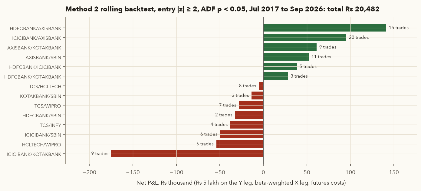
| Entry trigger | Trades | Win rate | Exits (stop / target / time) | Costs | Net P&L |
|---|---|---|---|---|---|
| |z| ≥ 2.5 (Varsity's preference) | 45 | 22.2% | 36 / 9 / 0 | ₹60,387 | −₹1,87,282 |
| |z| ≥ 2.0 | 108 | 40.7% | 63 / 43 / 2 | ₹1,44,105 | +₹20,482 |
- At 2.5 SD, the stop at 3 SD is only half an SD away. Pairs that diverge that far usually keep diverging, so 80% of trades were stopped out.
- HDFCBANK/ICICIBANK, the pair Varsity uses, qualified on only 16.4% of the 2,268 days (ADF p < 0.05). On no day was it both cointegrated and beyond 2.5 SD, and on only 5 days was it beyond 2 SD. It produced 5 trades in 9 years (net +₹38,506).
- Example win: signal 28 Feb 2025, Y = ICICI, X = HDFC, β 1.188, z −2.08, ADF p 0.021. Long 413 ICICI at 1,210.50, short 491 HDFC at 869.90 on 3 Mar. Target reached; exit 6 Mar at 1,227.95 / 843.50. ICICI +₹7,208, HDFC +₹12,956, costs ₹1,546, net +₹18,618 in 3 days.
- Example loss: signal 3 Oct 2025, z −2.06, β 1.381. Long ICICI at 1,371.00, short HDFC at 971.90 on 6 Oct. HDFC rallied, z reached −3.31, and the position was stopped on 21 Oct: net −₹13,913.
Pair trading is a real technique and teaches excellent statistical habits. On liquid Indian large caps, with daily data, current STT and honest rolling statistics, it was roughly break-even over nine years at best. Use the method to think about relative value (for example, "is this bank cheap relative to its peer?"). If you trade it, use small size, check the ADF test every day, and stop as soon as the relationship breaks.
13. Calendar spreads as a system
Varsity's calendar-spread chapter treats the price difference between two futures expiries of the same stock like a pair. Because both legs are the same underlying, this one really is close to market neutral. Steps: compute the daily difference (next month − current month), its mean and SD; sell the spread (sell the farther contract, buy the nearer) when it rises above mean + 1 SD; buy the spread when it falls below mean − 1 SD; close as it returns towards the mean. Varsity's example used SBIN.
Varsity's SBIN calendar spread, 2026 edition
The data comes from NSE's bhavcopy, the official end-of-day file listing every contract's open, high, low, close, settlement price, open interest and lot size.
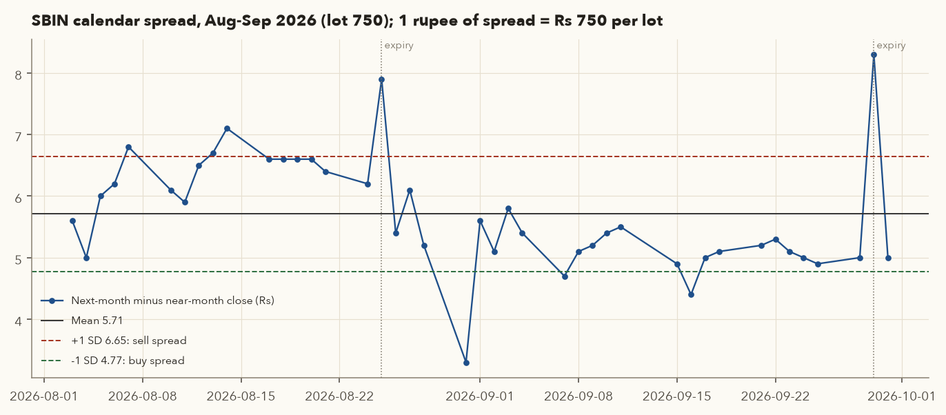
- Mean spread ₹5.71, SD ₹0.94 → sell above 6.65, buy below 4.77. Lot 750, so each ₹1 of spread is ₹750 per lot.
- Five signals (exit at the first close back inside the band, within the same expiry pair): gross ₹525, ₹75, ₹1,725, ₹300, ₹450 = ₹3,075.
- Each round trip has four legs of futures charges, about ₹935–₹1,021 per lot here. STT alone on one sell leg is 0.05% × ₹967.20 × 750 = ₹362.70. Total costs ₹4,902 → net −₹1,827. Break-even move ≈ ₹1.31 of spread, larger than one SD.
- Spread spikes on expiry days (₹7.9 on 25 Aug, ₹8.3 on 29 Sep) are mechanical: the near contract converges to spot. Avoid signals there.
- Honest caveat: the mean and SD use the whole 42-day window (look-ahead), and 42 days is a tiny sample.
After the April 2026 STT increase on futures, small mispricings like these rarely cover four legs of costs for a retail trader.
14. Momentum portfolios
Varsity's final system is a portfolio, not a trade. Momentum is the tendency of recent winners to keep outperforming for a while. Varsity's steps: (1) define a tracking universe (it suggests 150–200 stocks, e.g. from the BSE 500, for a 12–15 stock portfolio); (2) get clean, corporate-action-adjusted prices; (3) compute 12-month returns; (4) rank them; (5) buy the top names in equal weight; (6) rebalance monthly, selling names that drop out and buying new entrants.
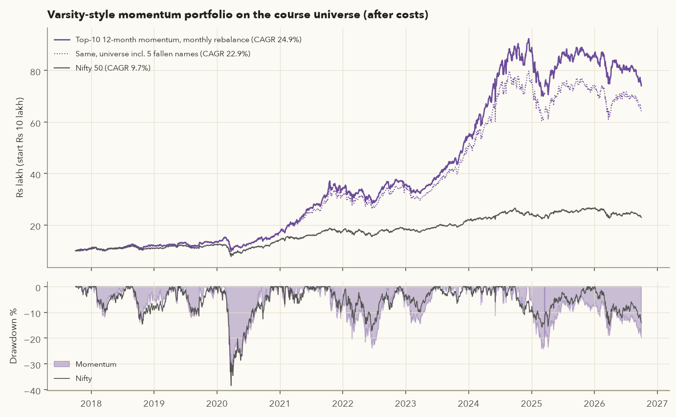
| Calendar year | 2018 | 2019 | 2020 | 2021 | 2022 | 2023 | 2024 | 2025 | 2026 YTD |
|---|---|---|---|---|---|---|---|---|---|
| Momentum (net) | +10.2% | +11.1% | +27.9% | +98.7% | +4.9% | +52.7% | +60.3% | −1.4% | −14.2% |
| Nifty | +3.2% | +12.0% | +14.9% | +24.1% | +4.3% | +20.0% | +8.8% | +10.5% | −13.4% |
Gross of costs the CAGR was 26.3%. With the five fallen names in the universe it was still 22.9%, because momentum rarely holds stocks while they collapse. But the universe still contains the 2026 survivors, which were picked partly because they had enormous runs (TRENT, BEL, HAL, DIXON, ADANIENT). A momentum system run on a 2017 list of 150–200 stocks, many of them later losers, would show a much smaller number. Note also 2025 (−1.4% vs Nifty +10.5%): momentum suffers when leadership changes suddenly. The top 10 by 12-month return at the 31 Aug 2026 rebalance were TITAN (+41.1%), POLYCAB, SBIN, NESTLEIND, SUNPHARMA, AXISBANK, ADANIENT, BAJFINANCE, TATASTEEL and LT (+12.0%). That is a historical illustration of how the rule works, not a recommendation.
Of everything tested here, the two that held up best were both slow, diversified, rules-based portfolio approaches: trend-following with cut losses (System B) and monthly momentum. Even those need a point-in-time universe test before you trust them. Chapter 17 builds your personal framework from these pieces.
15. Try it yourself
These snippets need a copy of the course repository (its data/ folder holds the price files) and Python with pandas and numpy; the setup steps are in the repository's framework/README.md. Save a snippet as a .py file and run it from the repository's root folder (for example .venv/bin/python snippet.py), because the file paths below are relative to that folder. Each one reproduces a number from this chapter.
15.1 A complete honest backtest in 20 lines (System A)
import pandas as pd, numpy as np
D = "data/ohlc/"                      # relative to the repository root
df = pd.read_csv(D + "IDX_NSEI.csv", index_col=0, parse_dates=True)
c, o = df["Close"], df["Open"]

# 1. signal decided at the CLOSE of day t (1 = want to be long)
sig = (c.rolling(50).mean() > c.rolling(200).mean()).astype(int)
# 2. position held from the OPEN of day t+1  (the shift is what prevents look-ahead)
pos = sig.shift(1).fillna(0)
prev = pos.shift(1).fillna(0)                     # position carried overnight into today
# 3. returns: overnight (close->open) belongs to yesterday's position, intraday (open->close) to today's
r_co = (o / c.shift(1) - 1).fillna(0)
r_oc = c / o - 1
gross = (1 + prev * r_co) * (1 + pos * r_oc) - 1
# 4. costs as a fraction of value traded: buy 0.1187% / sell 0.1037% (STT, stamp, exchange, SEBI, GST) + 0.05% slippage
buy, sell = (pos - prev).clip(lower=0), (prev - pos).clip(lower=0)
net = gross - buy * (0.001187 + 0.0005) - sell * (0.001037 + 0.0005)
# 5. equity curve and two headline metrics
eq = (1 + net.loc["2017-07-24":]).cumprod()
yrs = (eq.index[-1] - eq.index[0]).days / 365.25
print(f"CAGR {eq.iloc[-1] ** (1 / yrs) - 1:.2%}   max drawdown {(eq / eq.cummax() - 1).min():.2%}")
Expected output: CAGR 2.52% max drawdown -42.85%. Now change 50/200 to 20/50, or set the costs to zero, and see how much each choice matters.
15.2 See look-ahead bias with your own eyes
import pandas as pd
D = "data/ohlc/"                      # relative to the repository root
c = pd.read_csv(D + "IDX_NSEI.csv", index_col=0, parse_dates=True)["Close"].loc["2017-01-01":]
sig = (c > c.rolling(20).mean()).astype(int)
r = c.pct_change()
buggy = (1 + sig * r).loc["2017-07-24":].cumprod()             # WRONG: today's signal earns today's return
right = (1 + sig.shift(1) * r).loc["2017-07-24":].cumprod()    # signal known at close, earns from tomorrow
for name, eq in [("buggy", buggy), ("shifted", right)]:
    yrs = (eq.index[-1] - eq.index[0]).days / 365.25
    print(f"{name:8s} CAGR {eq.iloc[-1] ** (1 / yrs) - 1:6.1%}")
Expected: the buggy version shows roughly 46% a year, the shifted one roughly 8%. One missing .shift(1) is worth almost 38 percentage points of imaginary return.
15.3 Regression, error ratio and an ADF t-statistic in numpy (Method 2)
import numpy as np, pandas as pd
D = "data/ohlc/"                      # relative to the repository root
def close(sym):
    d = pd.read_csv(D + f"{sym}.csv", index_col=0, parse_dates=True)
    return d.loc[~((d.Volume == 0) & (d.High == d.Low)), "Close"]   # drop holiday filler bars
px = pd.DataFrame({s: close(s) for s in ["TCS", "INFY"]}).dropna().iloc[-200:]
y, x = px["TCS"].values, px["INFY"].values
X = np.column_stack([np.ones(len(x)), x])
(c, m), *_ = np.linalg.lstsq(X, y, rcond=None)          # y = m*x + c
e = y - (m * x + c)                                     # residuals
se = np.sqrt(e @ e / (len(y) - 2))                      # standard error of the regression
se_c = np.sqrt(se**2 * np.linalg.inv(X.T @ X)[0, 0])    # standard error of the intercept
print(f"slope {m:.4f}  intercept {c:.2f}  std err {se:.2f}  error ratio {se_c / se:.4f}  z today {e[-1] / se:+.2f}")
# ADF t-statistic on the residuals (1 lag): regress de_t on e_{t-1} and de_{t-1}
de = np.diff(e)
Z = np.column_stack([np.ones(len(de) - 1), e[1:-1], de[:-1]])
b, *_ = np.linalg.lstsq(Z, de[1:], rcond=None)
u = de[1:] - Z @ b
cov = (u @ u / (len(u) - 3)) * np.linalg.inv(Z.T @ Z)
print(f"ADF t-stat {b[1] / np.sqrt(cov[1, 1]):.2f}  (pair needs roughly < -3.3 for 5% significance)")
Expected: slope 1.8235, intercept 211.31, std err 80.16, error ratio 0.4388, z +0.33, ADF t −2.90. Swap in WIPRO and INFY and you should get an ADF t of about −3.33.
15.4 Exercises with the full chapter code
- The full chapter script is
course/scripts/ch12_figures.pyand the helper library iscourse/scripts/ch12_lib.py. Every number in this chapter is written todata/extra/ch12_results.json, and trade logs go todata/extra/ch12_donchian_trades.csv,ch12_rsi2_trades.csvandch12_pair_trades_entry2.0.csv. - Open the Donchian trade log in pandas and compute expectancy by year:
t.groupby(pd.to_datetime(t.exit_date).dt.year)["r"].mean(). How stable is it? - With the framework:
python -m framework.backtest_cli donchian_trend --risk 0.5 --out my_reportsand compare max drawdown at 0.5% vs 1% risk. (--outkeeps your experiment out offramework/reports/, whose files Chapter 17 quotes.)
16. From backtest to live: paper trading and the go-live checklist
Before you call a backtest "done"
- The hypothesis is written in one sentence, and I can say who is on the other side of my trades.
- All five components (universe, entry, exit, size, portfolio rules) are written precisely enough for someone else to code them identically.
- Signals use only completed bars; fills are at the next open (or worse); every indicator was checked for look-ahead (the result is not "too good to be true").
- Costs use current rates (delivery STT 0.1% both sides; futures STT 0.05% on sell since 1 Apr 2026; stamp, exchange, SEBI, GST, DP) plus slippage, and the system survives double slippage.
- The universe is point-in-time, or I have tested with known losers added and treat the result as an upper bound.
- At least 100 trades (ideally several hundred), spread over bull, bear and sideways markets.
- Parameters were fixed before testing; neighbouring parameters give similar results (a plateau, not a spike).
- An untouched out-of-sample period or a walk-forward test confirms the edge.
- A random-entry or buy-and-hold benchmark has been beaten after costs and taxes.
- I know the worst drawdown, the longest losing streak and the Monte-Carlo drawdown range, and I can live with 1.5× that.
Paper trading (1–3 months)
- Run the scan at the same time every day (for example 4:00–8:00 pm) and record every signal, even the ones you would not "like" to take.
- Record the price you would really have got (the next day's open), not the price you hoped for.
- Compare paper results with what the backtest code produces for the same dates. Differences mean bugs or unrealistic assumptions.
- Note practical frictions: data delays, corporate actions, holidays, results days, circuit limits, F&O ban periods for futures.
Going live, small
- Start at 25–50% of the planned risk per trade (e.g. 0.25–0.5% instead of 1%).
- Keep a trade journal (Chapter 11): signal, fill, slippage vs plan, exit reason, R-multiple, and any rule broken.
- After 20–30 live trades, compare win rate, average R and slippage with the backtest's range, not with its average.
- Pre-commit a kill switch, e.g. stop trading the system if the drawdown exceeds 1.5× the backtest maximum or the live expectancy after 50 trades is below the backtest's 5th percentile.
- Review quarterly. Re-run the backtest with new data, but do not re-optimise after every losing month.
- Size up only after the system has behaved as expected through at least one meaningful drawdown.
A backtest is a simulation of the past, not a forecast. Markets change, costs and taxes change (STT on futures more than doubled in 2026), and your own discipline in a drawdown is the variable no backtest captures. Never risk money you cannot afford to lose. Be especially careful with leveraged futures, where losses can exceed your margin.
17. Key takeaways
- A trading system is a complete written process (universe, entry, exit, size, portfolio rules) that can be tested. Tips, gut feel and one-off deductions are not systems.
- Design in order: hypothesis → rules → backtest → robustness → paper → small live → scale. If a test fails, go back to the hypothesis, not to the parameters.
- Signal at the close, fill at the next open, charge real Indian costs and slippage. One missing
shift(1)turned a 2.75% system into a fake 45.8% one. - Judge systems with several metrics together: CAGR, max drawdown, Sharpe/Sortino, Calmar, profit factor, expectancy in R, trade count, holding period and exposure. Always compare with buy-and-hold.
- On 2017–2026 data: the Nifty 50/200 crossover (2.5% CAGR) lost to buy-and-hold (9.3%); RSI(2) mean reversion was destroyed by costs (−6.6%); the 55-day breakout made 12.1%, but random entries did as well and adding five fallen stocks cut it to 8.3%.
- Survivorship bias, overfitting, look-ahead, costs and small samples all make backtests look better than reality. Even 424 trades left a confidence interval that included zero.
- Pair trading (Varsity Method 1 and 2) needs a stable, cointegrated relationship. Test the residuals with ADF using Engle-Granger critical values (≈ −3.3 at 5%), compute stats on a rolling past window, and size by β with real lot sizes. In 2017–2026 it was roughly break-even after costs.
- Calendar spreads now struggle to cover four legs of futures costs. Momentum portfolios looked strong but inherit our universe's survivorship bias.
- Go live small, journal everything, compare against the backtest's range, and set a kill switch in advance.
18. Quiz and exercises
Q1. A friend's system: "Buy strong stocks when the market looks good; sell when it looks weak." Which of the five components is properly defined?
Q2. Nifty closes above its 20-day SMA on Monday. In an honest backtest, which day's return does that signal earn first, and from what price?
Q3. A system turned ₹10 lakh into ₹28.55 lakh in 9.1855 years with a max drawdown of −33.46%. Compute CAGR and Calmar.
Q4. Win rate 30.4%, average win +3.60R, average loss −1.17R. What is the expectancy, and is a 30% win rate a problem?
Q5. RSI(2) had a 63.6% win rate and +0.17% average trade before costs, yet lost 6.6% a year after costs. Explain using the cost of a ₹1 lakh delivery round trip.
Q6. Why is a backtest of System B on our 37 stocks biased, and in which direction? What fixes it?
Q7. Out of 100 SMA pairs, 70/100 had the best Sharpe in 2009–2017 (0.49). Out-of-sample it ranked 76th. What does this tell you, and what would you do instead?
Q8. The ICICI/HDFC ratio is 1.8778, the 2-year mean is 1.5416 and SD 0.16358. Compute the density value. Which Method 1 trade does it trigger, and what is wrong with using these statistics?
Q9. Regressing A on B gives SE(intercept) 42.17 and SE 65.71. B on A gives 130.70 and 90.16. Which is Y? The residual ADF t-stat is −1.88. Trade?
Q10. WIPRO (Y) vs INFY (X) has β = 0.1413. WIPRO's lot is 3,000 and INFY's is 400. How many lots of each for a beta-neutral long-pair trade, and which side do you buy?
Q11. Your paper-traded breakout system has lost money on its first 30 trades (average −0.5R), while the backtest says +0.28R. Should you abandon it?
Q12. Exercise: the SBIN calendar spread's mean is ₹5.71 and SD ₹0.94, and a round trip costs about ₹980 per lot (lot 750). What is the minimum spread move to break even, and what does that imply for a ±1 SD system?
19. Sources
Sources: Zerodha Varsity Module 10 "Trading Systems": module page;
1. What to expect?;
2. Pair Trading logic;
3. PTM1 C1 – Tracking Pairs;
4. PTM1 C2 – Pair stats;
5. PTM1 C3 – Pre trade setup;
6. PTM1 C4 – The Density Curve;
7. PTM1 C5 – The Pair Trade;
8. PTM2 C1 – Straight line equation;
9. PTM2 C2 – Linear Regression;
10. PTM2 C3 – The Error Ratio;
11. PTM2 C4 – The ADF test;
12. Trade Identification;
13. Live Example 1;
14. Live Example 2;
15. Calendar Spreads;
16. Momentum Portfolios.
Varsity Module 9 "Risk Management & Trading Psychology": Equity Curve, Expected Returns.
Charges: Zerodha charges page (checked 2 Oct 2026: delivery STT 0.1% buy and sell, futures STT 0.05% sell, NSE 0.00307% / 0.00183%, SEBI ₹10/crore, stamp 0.015% / 0.002%, DP ₹15.34). Risk-free rate ≈ 5.5% (91-day T-bill ≈ 5.52%, RBI, Oct 2026, as recorded in framework/config.py).
Data: daily OHLCV for 37 NSE stocks and Nifty 50, NSE via Yahoo Finance (data/ohlc/, to 30 Sep 2026); Nifty history from 2007 and five delisted/collapsed stocks (YESBANK, ZEEL, SAMMAANCAP, IDEA, INDUSINDBK) downloaded with yfinance to data/extra/ch12_*_yf.csv; SBIN futures and F&O lot sizes from the NSE F&O UDiFF bhavcopy, Aug–Sep 2026 (data/fno/).
Code (in the course repository): course/scripts/ch12_figures.py, course/scripts/ch12_lib.py; all numbers in data/extra/ch12_results.json. Engle-Granger critical values were simulated (4,000 pairs of independent random walks, n = 200).