
Valuation
1. What you'll learn and why it matters
Chapters 6 and 7 taught you to judge whether a business is good. This chapter answers the next question: is the stock worth what the market is asking for it? A wonderful company bought at a silly price can still lose you money for years. You will meet a real case below: Asian Paints in January 2022.
By the end of this chapter you will be able to:
- Explain the difference between price and value, and why valuation gives you a range, not one exact number.
- Move money through time with present value (PV), future value (FV) and net present value (NPV).
- Build a discounted cash flow (DCF) model from scratch: free cash flow to the firm (FCFF), cost of equity from CAPM with a beta you compute yourself, WACC, terminal value, enterprise value, equity value and value per share.
- Run a sensitivity table and apply a margin of safety.
- Run a reverse DCF: find the growth rate today's price is quietly assuming.
- Use relative valuation properly: P/E bands, P/S, P/B for banks, EV/EBITDA, PEG, and know when each one fits.
- Spot the classic valuation traps (garbage-in, terminal-value dominance, cyclicals at peak earnings, one-off gains, look-ahead bias, value traps), each shown with a real Indian example.
- Read the market's overall valuation (Nifty P/E, earnings yield vs the 10-year G-sec) and build a watchlist with buy-zone prices.
Long-term investor: valuation decides your returns as much as business quality does. Overpay and you can earn nothing for years even while the company grows.
Swing trader: you will not run a DCF for a three-week trade. But knowing that a stock trades at 80x earnings tells you how hard it can fall on a small earnings miss, and an index P/E at the bottom of its range tells you something about the backdrop for your trades.
Futures trader: leverage magnifies valuation risk. A richly valued stock can gap down 10–15% on results day, and with futures you feel that several times over. Valuation context tells you where the air pockets are.
The main real examples in this chapter: a full DCF of Pidilite Industries; reverse DCFs of Asian Paints and ITC (plus Pidilite); a dividend discount model of ITC; P/E bands of Pidilite, Asian Paints, ITC and TCS; the cyclical P/E trap at Tata Steel; P/B for five large banks; EV/EBITDA across paints, metals and cement; and the Nifty 50's own valuation. Financials are consolidated, from screener.in pages fetched on 2 Oct 2026 (FY26 annual results plus the June-2026 quarter). Prices are NSE closes on 30 Sep 2026.
Every valuation in this chapter is a worked example built on stated assumptions. Change an assumption and the answer changes, sometimes a lot. Nothing here is a recommendation to buy or sell any security. Equity investing can lose money, and leveraged products can lose more than you put in.
2. Price is not value
Price is what you pay: the last traded number on the screen. It changes every second and reflects the mood, flows and news of the moment. Value (also called intrinsic value or fair value) is what the business is worth to an owner, based on the cash it is expected to produce over its life. Value changes slowly, as the business itself changes.
Varsity puts it simply: an investment works best when a great business is bought at a great price, and even a mediocre business can be a good investment if the price is low enough. Valuation is the third stage of equity research. Stage one asks whether you understand and like the business, stage two checks its financial performance (chapters 6–7), and stage three asks whether the price makes sense.
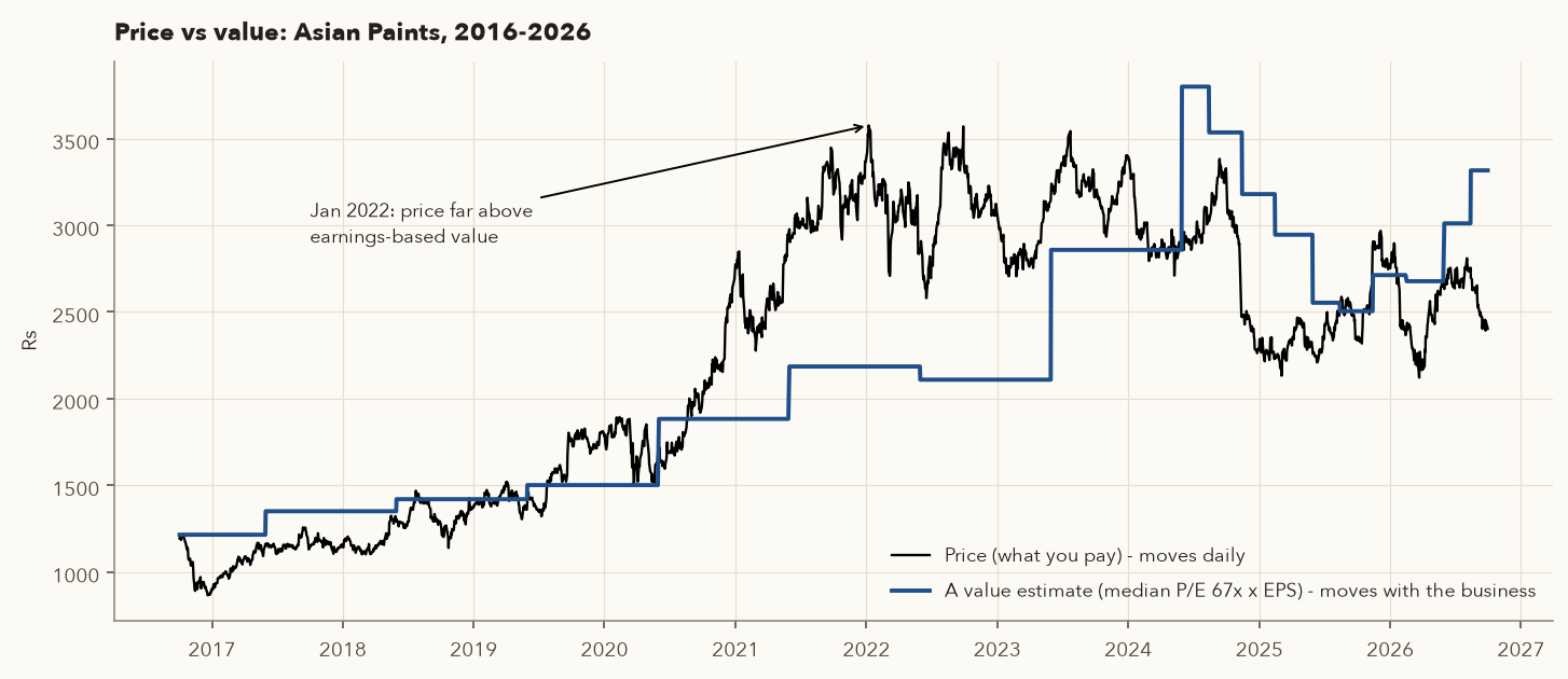
A great company, an expensive price
- On 7 Jan 2022 Asian Paints closed at ₹3,576.3. Its trailing P/E was 109.3x, well above its own 10-year median of about 67x.
- The business kept growing. EPS went from ₹31.59 (FY22) to ₹45.09 (FY26), up 42.7%.
- The stock did not follow. On 30 Sep 2026 it closed at ₹2,402.6, down 32.8% from that January 2022 close.
- The gap came from the multiple: the P/E fell from 109x to about 48x. The business did fine. The buyer in January 2022 overpaid.
Valuation methods try to estimate value so you can compare it with price:
- Price well below value: possibly undervalued. Worth researching, never an automatic buy.
- Price near value: fairly valued. You earn roughly the business's own return from here.
- Price well above value: overvalued. Future returns depend on things going better than expected.
Every value estimate rests on assumptions about the future. Varsity suggests treating your DCF output as a band of ±10% (a "modelling error" band) instead of one exact number, and buying only when the price is comfortably below that band. We will do exactly that for Pidilite.
3. Time value of money: PV, FV and NPV
₹100 today is worth more than ₹100 a year from now, for two reasons: you could invest today's ₹100 and earn a return (opportunity cost), and future money is uncertain. So money received at different times cannot be added up directly. It first has to be moved to the same point in time.
- Compounding moves money forward in time. The result is the future value (FV).
- Discounting moves money backward in time. The result is the present value (PV).
- \(PV\)
- Present value: what the money is worth today, in ₹.
- \(FV\)
- Future value: what the money will be worth (or the amount you will receive) at the end of \(n\) periods, in ₹.
- \(r\)
- The rate per period, written as a decimal (7.18% = 0.0718). It is your opportunity cost, the return you could earn elsewhere, also called the "discount rate". In this chapter a period is one year, so \(r\) is a yearly rate.
- \(n\)
- The number of periods (here, years) between today and the future date.
- \((1+r)^{n}\)
- The small raised \(n\) is an exponent: multiply \((1+r)\) by itself \(n\) times. \(1.0718^{5} = 1.0718 \times 1.0718 \times 1.0718 \times 1.0718 \times 1.0718\).
How it works: each year the money grows by the factor \((1+r)\), so after \(n\) years it has grown by \((1+r)^{n}\). Compounding multiplies by that factor to go forward in time. Discounting divides by it to come back to today. The bigger \(r\) or \(n\), the smaller today's value of a future rupee.
Moving money through time
Use the 10-year Government of India bond (G-sec) yield on 30 Sep 2026, 7.18%, as a nearly risk-free rate.
- FV: ₹10,000 invested for 5 years at 7.18%: \(10{,}000 \times 1.0718^{5} = ₹14{,}143.89\).
- PV: ₹1,00,000 promised in 10 years, with a required return of 12% (a typical equity hurdle): \(1{,}00{,}000 / 1.12^{10} = ₹32{,}197.32\). The promise is worth less than a third of its face value today.
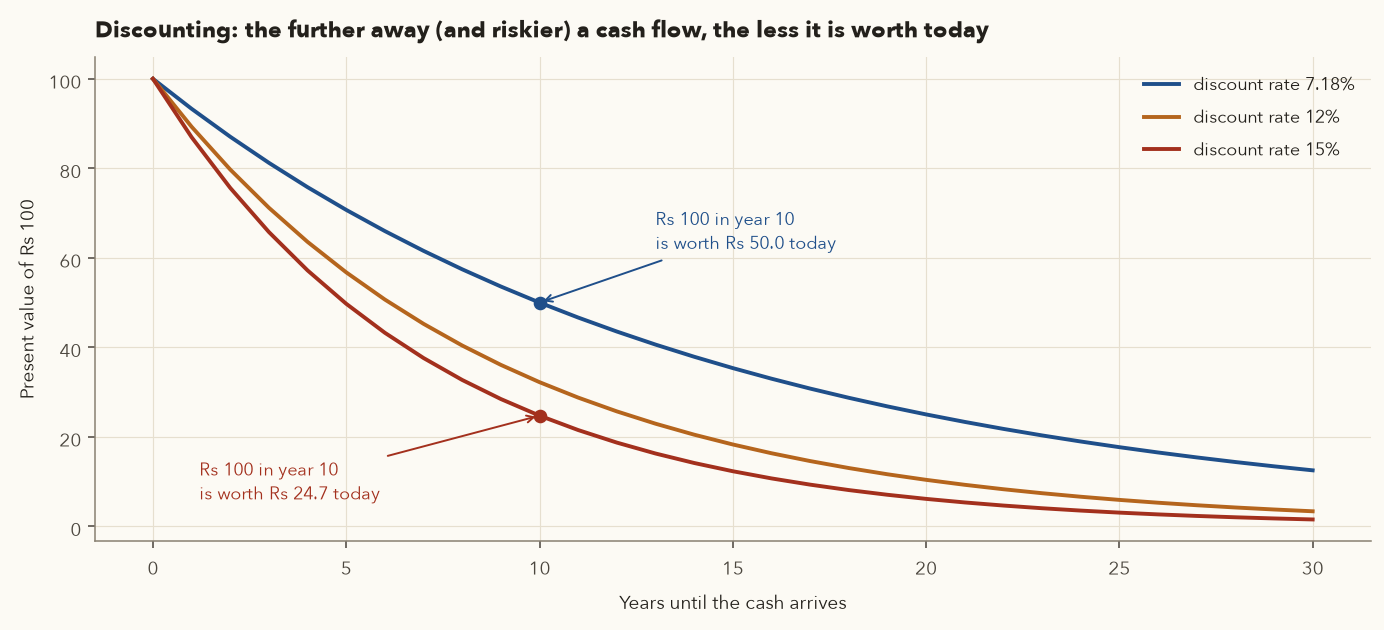
- Check: ₹100 due in 10 years is worth about ₹50 today at 7.18%, but only ₹24.7 at 15%. A higher discount rate means a lower present value.
Net present value (NPV)
When an asset produces a stream of cash flows, discount each one separately and add them up. That sum is the net present value. It is the most you should rationally pay today for that stream.
- \(\Sigma\)
- "Sigma" means add up: work out the fraction for \(t = 1\), then \(t = 2\), and so on up to \(t = n\), and add the results.
- \(t\)
- The year a cash flow arrives: 1 for one year from today, 2 for two years, and so on.
- \(CF_t\)
- The cash flow received in year \(t\), in ₹.
- \(n\)
- The last year in which a cash flow arrives.
- \(r\)
- The yearly discount rate, as a decimal (as in the formula above).
- \(NPV\)
- Net present value: the whole stream of cash flows expressed as one amount in today's ₹.
- Take each year's cash flow and divide it by \((1+r)^{t}\). This is the present-value formula above, applied once per year.
- Later cash flows are divided by a bigger number, so they count for less.
- Add up all the present values. The total is the most you should pay today for the whole stream.
What is a machine worth if it earns ₹5 lakh a year for 10 years?
Varsity's DCF primer uses a pizza machine that earns ₹5,00,000 a year for 10 years and is then worthless. We re-run it with the current G-sec yield of 7.18% as the opportunity cost.
- Total cash over 10 years: \(10 \times 5{,}00{,}000 = ₹50{,}00{,}000\). You should never pay more than this.
- PV of year 1's cash: \(5{,}00{,}000/1.0718 = ₹4{,}66{,}505\). PV of year 10's cash: \(5{,}00{,}000/1.0718^{10} = ₹2{,}49{,}938\).
- Sum of all ten PVs = NPV = ₹34,82,756. That is the most a buyer earning 7.18% elsewhere should pay. A lower price is a good deal, a price at NPV is a fair deal, and a higher price is a bad deal.
Replace the machine with a company and its cash flows with free cash flow, and you have a DCF.
4. Three ways to value a business
Varsity's financial-modelling module groups valuation methods into three families:
| Family | Idea | Typical tools | Best for |
|---|---|---|---|
| Relative (comparables) | Similar businesses should sell at similar multiples | P/E, P/S, P/B, EV/EBITDA, PEG | Quick checks, peer comparison, your stock's own history |
| Absolute (intrinsic) | Value = PV of future cash flows | DCF on FCFF or FCFE, dividend discount model | Stable, cash-generating businesses you understand |
| Option-based | Value depends on whether some event happens | Option-pricing logic (covered in options chapters) | Early-stage firms, R&D bets, mining or biotech outcomes |
Relative valuation is intuitive but has two weaknesses that Varsity points out. The whole sector can be mispriced (think of the dot-com bubble), and no two companies are truly identical. A firm with a 25% profit margin deserves a higher P/S than one with 15%. Absolute valuation forces you to write down every assumption, which is its strength, but the output is only as good as those assumptions.
Enterprise value vs equity value
Rearranging the balance sheet makes the two viewpoints clear. Assets = debt + equity. Split the assets into cash and operating assets and move cash to the other side:
- Operating assets
- Everything the business uses to run itself (plants, brands, inventory, receivables), i.e. all assets except surplus cash and investments. In ₹ crore.
- Debt
- Money owed to lenders: borrowings, including lease liabilities. In ₹ crore.
- Cash
- Cash, bank balances and surplus investments the business does not need to operate. In ₹ crore.
- Net debt
- Debt minus cash. If cash is larger than debt, net debt is negative and the company has net cash.
- Equity
- The shareholders' claim on the business.
How it works: the operating business is financed partly by lenders (net of the cash they could be repaid from) and partly by shareholders. So if you know the value of the whole operating business (enterprise value), you get the shareholders' part by subtracting net debt, or by adding net cash.
Example (from the Pidilite DCF in Section 8, ₹ crore): enterprise value 38,191 and net cash 4,232 (net debt of −4,232), so equity value = 38,191 + 4,232 = 42,423.
- Value the operating business (all the capital, from lenders and owners together) and you get enterprise value (EV). You discount free cash flow to the firm (FCFF) at the blended cost of all capital, the WACC.
- Value only the shareholders' part and you get equity value. You discount free cash flow to equity (FCFE) at the cost of equity.
- The bridge between them: Equity value = EV − debt + cash (and surplus investments). Divide by shares outstanding to get value per share.
5. Free cash flow: FCF, FCFF and FCFE
A business is worth the cash it can hand back to its owners. Profit is an accounting opinion; cash is a fact (chapter 6). The cash flow we discount is free cash flow: what is left after the company has paid its running costs and taxes and reinvested enough in fixed assets and working capital to keep growing.
- Cash from operations
- (CFO) The operating cash flow line of the cash flow statement: cash the business actually collected from running itself in the year, in ₹ crore.
- Capex
- Capital expenditure: money spent in the year on fixed assets (plants, machinery, stores), net of assets sold. From the investing section of the cash flow statement.
- FCFF
- Free cash flow to the firm: cash left for all providers of capital, lenders and shareholders together, after running costs, tax and reinvestment.
- FCFE
- Free cash flow to equity: cash left for shareholders only, after lenders have been paid interest and after any new borrowing or repayment.
- EBIT
- Earnings before interest and tax: operating profit after depreciation. EBITDA is the same figure before depreciation and amortisation as well.
- \(t\)
- The company's tax rate, as a decimal (26% = 0.26).
- D&A
- Depreciation and amortisation for the year: a non-cash accounting charge, added back.
- \(\Delta\)Working capital
- The Greek letter \(\Delta\) ("delta") means "change in". This is the increase in working capital (inventory + receivables − payables) over the year. An increase ties up cash, so it is subtracted. A decrease releases cash, so subtracting a negative number adds it back.
- Interest
- Interest paid to lenders in the year. Multiplying by \((1-t)\) gives its after-tax cost, because interest reduces the tax bill.
- Net borrowing
- New loans taken minus loans repaid during the year. Positive if debt went up.
- Simple FCF is the quick version: take operating cash flow straight from the cash flow statement and subtract capex.
- FCFF builds the same idea from the profit and loss account: after-tax operating profit, plus the non-cash D&A, minus cash tied up in working capital, minus capex. Discount it at WACC to get enterprise value.
- FCFE starts from FCFF, takes off what lenders received (after-tax interest) and adds any net new borrowing. Discount it at the cost of equity to get equity value.
The logic behind each piece:
- EBIT × (1 − t), often called NOPAT, is the after-tax operating profit the business would earn if it had no debt. We start from EBIT, not PAT, because interest belongs to the lenders, who are part of "the firm".
- + D&A: depreciation is a non-cash charge. The cash left when the asset was bought, and that purchase is captured in capex.
- − ΔWorking capital: a growing company ties up more cash in inventory and receivables.
- − Capex: spending on plants, machinery and stores is real cash out.
The tax shield
Interest is tax-deductible, so debt reduces a company's tax bill. Varsity's example: EBIT ₹700 cr, interest ₹70 cr, tax 25%. With the interest, tax is ₹157.5 cr. Without it, tax would be ₹175 cr. The ₹17.5 cr saved is the tax shield, and it is why the after-tax cost of debt is \(K_d(1-t)\). If you start from PAT instead of EBIT, add back interest × (1 − t), not the full interest. Both routes give the same FCFF.
Pidilite's free cash flow to the firm, line by line
- Operating profit (EBITDA, excluding other income) = 3,521; depreciation = 395. So EBIT = 3,521 − 395 = 3,126.
- Tax rate FY26 = 26%. NOPAT = 3,126 × (1 − 0.26) = 2,313.2.
- Add back D&A: 2,313.2 + 395 = 2,708.2.
- Capex (fixed assets purchased 593, minus assets sold 4) = 589. Working capital absorbed 51 (from the cash flow statement).
- FCFF = 2,708.2 − 589 − 51 = ₹2,068.2 cr. For comparison, the simple version, CFO − capex = 2,828 − 589 = ₹2,239 cr.
Why exclude "other income" (₹248 cr in FY26)? It is mostly interest and gains on Pidilite's ₹4,350 cr of treasury investments. We will add those investments to the valuation separately at the end. Counting both their income and their balance would double count them.
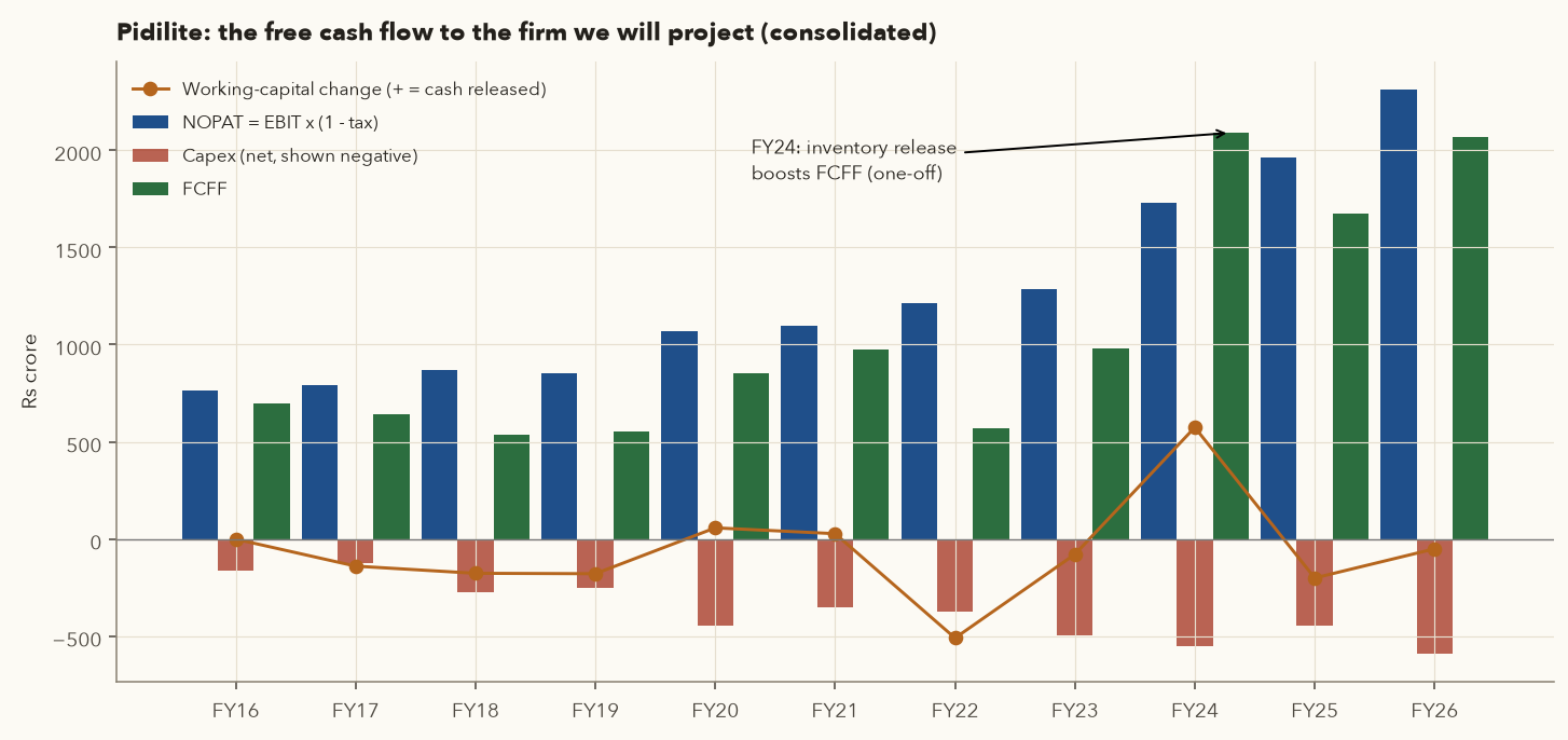
FCFF swings with working capital. Pidilite's last three years were ₹2,089.9 cr (FY24, helped by an inventory release), ₹1,672.2 cr (FY25) and ₹2,068.2 cr (FY26). Following Varsity, we use the three-year average, ₹1,943.5 cr, as the base year so one unusual year does not drive the whole valuation. Also watch acquisitions: in FY21 Pidilite spent about ₹2,061 cr in "other investing items" (largely buying a business). Growth bought this way is not free cash flow. A DCF that ignores acquisition spending overstates FCF for serial acquirers.
6. The discount rate: CAPM, beta and WACC
The discount rate is the return investors require for the risk they take. Lenders take less risk and accept a lower return. Shareholders are paid last and demand more.
6.1 Cost of equity with CAPM
- \(K_e\)
- Cost of equity: the yearly return shareholders require for holding this stock, in %.
- \(R_f\)
- The risk-free rate: the yearly return on a nearly riskless investment. We use the 10-year G-sec yield (7.18% on 30 Sep 2026).
- \(\beta\)
- Beta: how strongly the stock tends to move with the market. 1 = in line with the market, below 1 = less, above 1 = more. Computed from past returns (formula below).
- \(R_m\)
- The expected yearly return on the whole stock market, in %.
- ERP
- The equity risk premium, \(R_m - R_f\): the extra yearly return investors want for owning shares instead of government bonds. We use 7.0%.
How it works: start from what a riskless bond pays, then add a reward for risk. The reward is the market's risk premium scaled by beta, so a stock that swings more than the market must offer a higher expected return. The result, \(K_e\), is the discount rate for equity cash flows.
Risk-free rate. Varsity uses the 10-year G-sec yield as the proxy. On 30 Sep 2026 it was 7.18% (countryeconomy.com; Trading Economics shows 7.16%). It rose from 6.96% at the start of September 2026. We use \(R_f = 7.18\%\).
Equity risk premium. This is the extra return investors want for owning stocks instead of government bonds. Professor Aswath Damodaran's January 2026 update puts India's total ERP at 7.08%, and Indian valuation firm Incwert recommends 7.0% (range 6.5–7.5%) from January 2026. We use ERP = 7.0%. Varsity's older chapters instead assume a market return \(R_m\) of 8.5–12%. Either way, write the number down and justify it.
Beta. Beta measures how much a stock tends to move when the market moves. A beta of 1.2 means that, on average, a 1% Nifty move came with a 1.2% move in the stock. Compute it from your own data:
- \(R_{stock}\)
- The stock's return in each period, e.g. each week's % change in price (dividend-adjusted). A list of numbers, one per week.
- \(R_{market}\)
- The market index's return (here the Nifty 50) over the same weeks.
- \(\operatorname{Cov}\)
- Covariance: a measure of how much the two return series move together. Positive if the stock tends to rise in weeks when the market rises.
- \(\operatorname{Var}\)
- Variance: how much the market's returns spread out around their average. It is the covariance of the market with itself.
How it works: dividing "how much they move together" by "how much the market moves" gives the average stock move per 1% market move. It is the slope of the line through a scatter of stock returns against market returns. In a spreadsheet, SLOPE(stock returns, market returns) gives the same number.
Computing Pidilite's beta and cost of equity
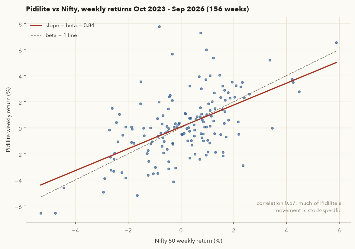
- Take weekly returns (Friday closes) for Pidilite (dividend-adjusted) and the Nifty 50 for the last 3 years: 156 weeks.
- Covariance of the two return series = 0.000248. Variance of Nifty returns = 0.000295.
- \(\beta = 0.000248 / 0.000295 = \mathbf{0.84}\). Pidilite has tended to move a little less than the market.
- \(K_e = 7.18\% + 0.84 \times 7.0\% = \mathbf{13.06\%}\).
| Stock | β 2y | β 3y | β 5y | Correlation (3y) | \(K_e\) = 7.18% + β(3y) × 7% |
|---|---|---|---|---|---|
| ITC | 0.45 | 0.51 | 0.65 | 0.37 | 10.75% |
| Pidilite | 0.86 | 0.84 | 0.91 | 0.57 | 13.06% |
| Asian Paints | 0.91 | 0.90 | 0.90 | 0.51 | 13.48% |
| TCS | 0.96 | 0.95 | 0.92 | 0.52 | 13.83% |
| HDFC Bank | 0.98 | 0.97 | 1.03 | 0.64 | 13.97% |
| Tata Steel | 1.26 | 1.24 | 1.23 | 0.59 | 15.86% |
| Trent | 1.32 | 1.27 | 1.27 | 0.38 | 16.07% |
| Adani Enterprises | 1.51 | 1.50 | 1.60 | 0.51 | 17.68% |
Weekly returns to 30 Sep 2026 vs the Nifty 50. Beta changes with the window: ITC's ranges from 0.45 to 0.65. Use a few windows and pick a sensible middle.
Two refinements you will meet in research reports. (1) Adjusted beta: raw betas tend to drift towards 1 over time, so many data providers report \(\beta_{adj} = 0.67\,\beta_{raw} + 0.33\). For Pidilite: \(0.67 \times 0.84 + 0.33 = 0.89\), which lifts \(K_e\) from 13.06% to about 13.4%. (2) Levered vs unlevered beta: a stock's beta contains business risk plus the extra risk from its debt. To compare companies with different debt levels, analysts strip debt out, \(\beta_U = \beta_L / [1 + (1-t)\,D/E]\), and put the target company's own debt back in. Tata Steel (debt/equity 0.40 at market value) has an unlevered beta of about \(1.24 / (1 + 0.7483 \times 0.40) = 0.95\). Most of its above-market beta comes from leverage. We use raw betas in this chapter to keep the arithmetic visible.
6.2 Cost of debt and WACC
- WACC
- Weighted average cost of capital: the blended yearly return required by all the company's investors, lenders and shareholders together, in %. It is the discount rate for FCFF.
- \(E\)
- Market value of equity: the market cap (share price × shares outstanding), in ₹ crore.
- \(D\)
- Debt: total borrowings, including lease liabilities, in ₹ crore.
- \(\frac{E}{D+E},\ \frac{D}{D+E}\)
- The weights: the share of total capital that comes from shareholders and from lenders. They add up to 1.
- \(K_e\)
- Cost of equity, from CAPM above.
- \(K_d\)
- Pre-tax cost of debt: roughly interest paid in the year ÷ average borrowings over the year, in %.
- \(t\)
- Tax rate. India's concessional corporate rate is 22% + 10% surcharge + 4% cess = 25.17%. It sat in section 115BAA of the Income-tax Act, 1961. From tax year 2026-27 the Income-tax Act, 2025 carries the same regime in section 200, at the same rates (checked Oct 2026). Most large listed companies have opted for it, which is why their reported tax rates cluster around 25–26%.
- Work out the after-tax cost of debt, \(K_d(1-t)\). Interest is tax-deductible, so debt costs less than its headline rate (the tax shield above).
- Multiply each cost by its weight: equity's share of capital × \(K_e\), and debt's share × after-tax \(K_d\).
- Add the two. A company with almost no debt has a WACC close to its cost of equity.
WACC for an almost debt-free company
- E = ₹1,465.1 × 101.45 cr shares = ₹1,48,628 cr. D = borrowings FY26 = ₹417 cr (mostly lease liabilities).
- Weights: E/(D+E) = 99.72%, D/(D+E) = 0.28%.
- \(K_d\) = interest ₹54 cr ÷ average borrowings ₹435.5 cr = 12.40%. After tax: 12.40% × (1 − 0.2517) = 9.28%.
- WACC = 0.9972 × 13.06% + 0.0028 × 9.28% = 13.05%. We round to 13.0%. With almost no debt, WACC ≈ cost of equity.
WACC when debt really matters
- E = ₹184.3 × 1,246.0 cr shares = ₹2,29,636 cr. D = ₹92,382 cr. Weights: equity 71.3%, debt 28.7%.
- \(K_d\) = interest ₹7,167 cr ÷ average borrowings (₹94,801 + ₹92,382)/2 = 7.66%. After tax: 5.73%.
- β = 1.24, so \(K_e\) = 7.18% + 1.24 × 7% = 15.86%.
- WACC = 0.713 × 15.86% + 0.287 × 5.73% = 12.95%. Cheap, tax-deductible debt pulls WACC well below the cost of equity. But more debt also raises equity risk (higher beta), so you cannot lower WACC forever by borrowing.
7. Terminal value: Gordon growth and exit multiple
We cannot forecast cash flows year by year forever. The standard approach forecasts explicitly for 5–10 years, then assumes the company settles into steady growth at rate \(g\) forever. The value of all cash flows after the forecast period, measured at the end of year \(N\), is the terminal value (TV).
- \(N\)
- The last year of the explicit forecast (10 in the Pidilite model).
- \(FCF_N\)
- The free cash flow forecast for year \(N\), in ₹ crore. \(FCF_N \times (1+g)\) is the first cash flow after the forecast, in year \(N+1\).
- \(g\)
- Terminal growth: the yearly rate at which cash flow is assumed to grow forever after year \(N\), as a decimal (5% = 0.05).
- \(r\)
- The discount rate: WACC if you are discounting FCFF.
- \(TV_N\)
- Terminal value: the value, measured at the end of year \(N\), of all cash flows from year \(N+1\) onwards, in ₹ crore.
- \(PV(TV)\)
- That terminal value brought back to today, using the present-value formula from Section 3.
- Grow the last forecast cash flow by one year: \(FCF_N \times (1+g)\).
- Divide by the gap \(r - g\). This one division adds up an endless stream of cash flows growing at \(g\) and discounted at \(r\).
- The answer is a value at year \(N\), not today, so divide by \((1+r)^N\) to get \(PV(TV)\).
- Only valid when \(r > g\). As \(g\) gets close to \(r\), the gap shrinks towards zero and the value explodes.
Intuition: a cash flow of ₹100 next year that grows 5% a year forever, discounted at 12%, is worth \(100 \times 1.05/(0.12-0.05) = ₹1{,}500\) at the end of year N. Nudge \(g\) to 6% and it becomes ₹1,766.7 (+18%). Nudge \(r\) down to 11% instead and it becomes ₹1,750. Small changes in the gap \((r - g)\) cause large changes in value. Keep this in mind for the sensitivity section.
No company can grow faster than the economy forever, or it would eventually become the economy. Varsity suggests a terminal growth near long-run inflation (3–5%). For an Indian company valued in rupees, many analysts allow up to roughly long-run nominal GDP growth, but anything above 6% needs a very strong argument. We use g = 5%. Always check that \(g\) is well below your discount rate.
The exit-multiple method
The alternative assumes the business is "sold" at the end of year N at a market multiple, for example \(TV_N = EBITDA_N \times\) EV/EBITDA multiple. It is popular with practitioners because it ties to market prices. But it imports today's market mood into a "fundamental" model. Always convert an exit multiple into the perpetual growth it implies and ask whether that growth is believable:
- \(TV_N\)
- The terminal value at the end of year \(N\) from the exit multiple, e.g. year-\(N\) EBITDA × the EV/EBITDA multiple, in ₹ crore.
- \(FCF_N\)
- The free cash flow forecast for year \(N\), in ₹ crore.
- \(r\)
- The discount rate (WACC), as a decimal.
- \(g_{implied}\)
- The perpetual growth rate that would make the Gordon formula above give the same \(TV_N\).
How it works: this is the Gordon formula rearranged to solve for \(g\) instead of \(TV\). Put in the terminal value the multiple gives you, and it tells you how fast cash flow must grow forever to be worth that much. If the answer is well above long-run GDP growth, the multiple is too generous.
Example (Pidilite, Section 8 step 5, ₹ crore): a 20x exit multiple gives \(TV_{10} = 1{,}90{,}950\), with \(FCF_{10} = 5{,}270\) and \(r = 0.13\). \(g = (1{,}90{,}950 \times 0.13 - 5{,}270)/(1{,}90{,}950 + 5{,}270) = 19{,}553.5/1{,}96{,}220 = 9.97\%\) a year, forever.
8. A complete DCF: Pidilite Industries
Pidilite (Fevicol, Dr. Fixit, M-Seal) is a near-debt-free consumer business with high returns on capital. That suits a DCF, because its cash flows are positive and fairly predictable. Here is the full model, step by step. All figures are in ₹ crore unless marked otherwise.
Step 1 — Growth assumptions and why
Growth rates below are compound annual growth rates (CAGR): \(\text{CAGR} = (\text{End}/\text{Start})^{1/\text{years}} - 1\). For example, sales of ₹5,361 cr (FY16) to ₹14,601 cr (FY26) is \((14{,}601/5{,}361)^{1/10} - 1 = 10.5\%\) a year. Over FY16–FY26 Pidilite's sales grew 10.5% a year and its EBIT 11.3% a year. FCFF grew 15.2% a year (three-year average FY16–18 to FY24–26), partly because margins expanded. For the explicit forecast we assume 12% a year for years 1–5 (a little above sales history and below the FCF history, on the view that margin expansion cannot repeat forever), then 9% for years 6–10 as the business matures, then 5% forever. This follows Varsity's two-stage approach (Varsity used 18%/10% for Amara Raja in 2014), but with growth anchored to the company's own track record.
Step 2 — Project and discount the cash flows
| Year | FY | Growth | FCFF | Discount factor \(1/1.13^t\) | Present value |
|---|---|---|---|---|---|
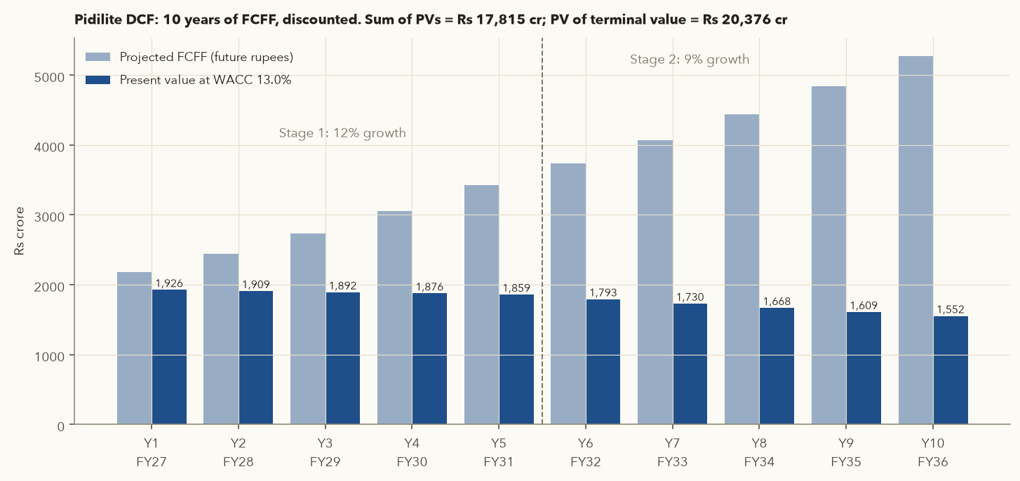
| 1 | FY27 | 12% | 2,176.7 | 0.8850 | 1,926.3 |
| 2 | FY28 | 12% | 2,437.9 | 0.7831 | 1,909.2 |
| 3 | FY29 | 12% | 2,730.4 | 0.6931 | 1,892.3 |
| 4 | FY30 | 12% | 3,058.1 | 0.6133 | 1,875.6 |
| 5 | FY31 | 12% | 3,425.0 | 0.5428 | 1,859.0 |
| 6 | FY32 | 9% | 3,733.3 | 0.4803 | 1,793.2 |
| 7 | FY33 | 9% | 4,069.3 | 0.4251 | 1,729.7 |
| 8 | FY34 | 9% | 4,435.5 | 0.3762 | 1,668.5 |
| 9 | FY35 | 9% | 4,834.7 | 0.3329 | 1,609.4 |
| 10 | FY36 | 9% | 5,269.8 | 0.2946 | 1,552.4 |
| Sum of PVs, years 1–10 | 17,815 | ||||
Example row: year 1 FCFF = 1,943.5 × 1.12 = 2,176.7, and its PV = 2,176.7 / 1.13 = 1,926.3. (The table is computed from the unrounded base, ₹1,943.43 cr. Starting from the rounded ₹1,943.5 moves later rows by ₹0.1–0.2 cr and leaves the per-share value at ₹418.2.) Notice how the PVs fall even though cash flows rise: discounting at 13% outruns 9–12% growth.
Step 3 — Terminal value
- \(TV_{10} = 5{,}269.8 \times 1.05 / (0.13 - 0.05) = \mathbf{69{,}167}\).
- \(PV(TV) = 69{,}167 / 1.13^{10} = 69{,}167 \times 0.2946 = \mathbf{20{,}376}\).
Step 4 — Enterprise value → equity value → per share
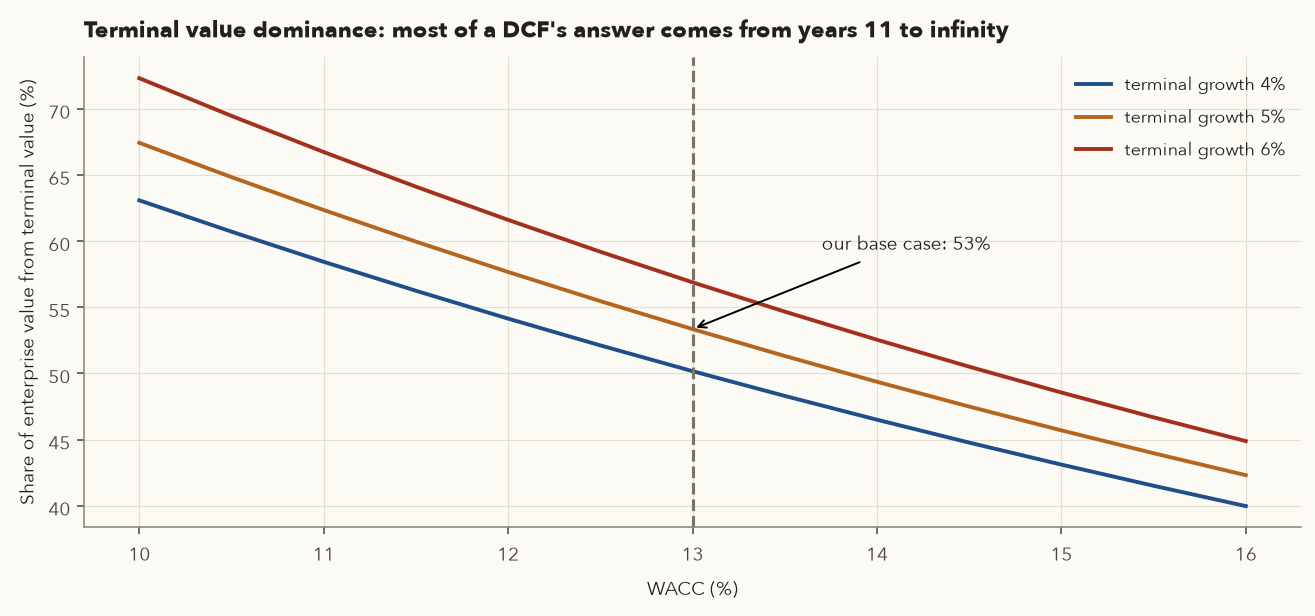
- Enterprise value = 17,815 + 20,376 = 38,191. The terminal value is 53.4% of it.
- Add cash and equivalents (299) and investments (4,350), and subtract borrowings including leases (417). Net cash = 4,232.
- Equity value = 38,191 + 4,232 = 42,423.
- Per share = 42,423 / 101.45 = ₹418.2.
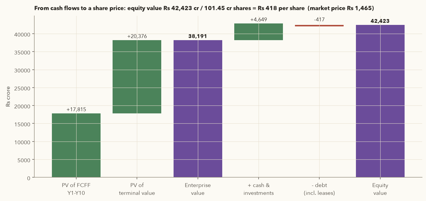
On 30 Sep 2026 Pidilite closed at ₹1,465.1, 3.5 times our base-case value. Varsity's ±10% modelling band is ₹376–₹460, and the price is far above it. Does that mean Pidilite is overvalued, or that the model is wrong? Possibly both, in part. Investors have paid 55–120x earnings for Pidilite for years, which implies they use a lower discount rate, expect faster growth for longer, or both. Section 10 turns the question around and asks what the price implies. That is usually more useful than arguing over one number.
Step 5 — Cross-check with an exit multiple
Suppose instead that at the end of FY36 the business is valued at 20x EBITDA, half its current ~40x. Grow FY26 EBITDA (₹3,521 cr) on the same path to ₹9,547 cr in year 10. Then \(TV = 20 \times 9{,}547 = 1{,}90{,}950\), its PV is 56,252, and value per share becomes ₹771.8. Now the terminal value is 75.9% of EV. Convert it into implied perpetual growth: \(g = (190{,}950 \times 0.13 - 5{,}270)/(190{,}950 + 5{,}270) = \mathbf{9.97\%}\) a year, forever. Even a "conservative" 20x exit multiple assumes Pidilite grows at almost 10% for eternity. That is how market multiples hide aggressive assumptions.
framework.fundamentals.dcf(fcf, growth, discount, terminal_growth, years, net_debt, shares) implements exactly this model. Pass growth as a list for multi-stage growth, and pass net cash as a negative net_debt. dcf(1943.5, [0.12]*5 + [0.09]*5, 0.13, 0.05, net_debt=-4232, shares=101.45) returns a per-share value of ₹418.2 and terminal_share_pct of 53.4. framework.fundamentals.reverse_dcf(...) solves for implied growth (section 10). python -m framework.invest PIDILITIND prints them next to the quality scorecard. You will combine everything in chapter 17.
9. Sensitivity and margin of safety
A DCF is a machine for turning assumptions into a number. To see how fragile that number is, vary the two most powerful inputs, the discount rate and terminal growth, and look at the whole grid.
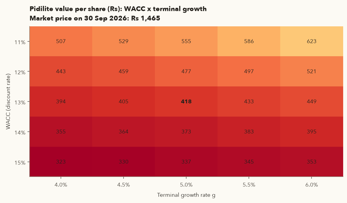
| WACC ↓ / g → | 4.0% | 4.5% | 5.0% | 5.5% | 6.0% |
|---|---|---|---|---|---|
| 11% | 507 | 529 | 555 | 586 | 623 |
| 12% | 443 | 459 | 477 | 497 | 521 |
| 13% | 394 | 405 | 418 | 433 | 449 |
| 14% | 355 | 364 | 373 | 383 | 395 |
| 15% | 323 | 330 | 337 | 345 | 353 |
Stage-1 growth matters just as much. Keeping WACC at 13% and terminal growth at 5%, with stage-2 growth 3 points below stage 1 (minimum 5%), value per share is ₹326 at 8% growth, ₹369 at 10%, ₹418 at 12%, ₹507 at 15%, ₹617 at 18% and ₹705 at 20%.
Margin of safety
Because the inputs are uncertain, insist on buying well below your estimate. That cushion is the margin of safety, a term from Benjamin Graham.
- Intrinsic value
- Your estimate of value per share, e.g. from the DCF (₹418.2 for Pidilite), in ₹.
- MOS
- The margin of safety: the discount you insist on, as a decimal (30% = 0.30).
- Buy price
- The highest price at which you would buy, in ₹ per share.
How it works: knock a fixed percentage off your estimate and only buy at or below the result. If your estimate turns out too high by less than the margin, you still have not overpaid. The less certain the estimate, the bigger the margin should be.
- Varsity's rule: build a ±10% band around the DCF value. Below the lower band, consider buying. Inside it, hold. Above the upper band, do not buy. For Pidilite the band is ₹376–₹460.
- A stricter rule uses 25–40% MOS. At 30%, Pidilite's buy price would be ₹293.
- Use a bigger MOS when the business is less predictable: cyclicals, high debt, short history, or governance questions.
They rarely trust the single output. They use it to learn which assumptions matter, to compare scenarios (bear / base / bull), and to ask "what must I believe to justify this price?" That last question is the reverse DCF, next.
10. Reverse DCF: what is the price assuming?
Instead of guessing growth and computing value, a reverse DCF takes the market price as given and solves for the growth rate (or the return) that makes the DCF value equal the price. Then you judge whether that growth is believable compared with the company's history and its industry.
- Market cap
- Today's share price × shares outstanding, in ₹ crore. This is the known "answer" the market has given.
- \(FCF_0\)
- The base-year free cash flow (the subscript 0 means "today's starting point"). Here it is the three-year average of CFO − capex, in ₹ crore.
- \(g\)
- The unknown: the yearly FCF growth for years 1 to 10 that the price implies.
- \(t\)
- The forecast year, 1 to 10. \(\Sigma\) adds up the ten discounted cash flows.
- \(r\)
- The discount rate. The examples below use each company's cost of equity. These companies have almost no debt, so it is close to their WACC.
- \(g_T\)
- Terminal growth after year 10, fixed at 5%.
- Net cash
- Cash + investments − borrowings, in ₹ crore.
- The first line is the present value of ten years of FCF, each one \(FCF_0\) grown by \(g\) for \(t\) years and discounted for \(t\) years.
- The second line adds the terminal value (Section 7) of year 10's cash flow, discounted back 10 years, and then the net cash.
- Everything is known except \(g\). Try a value of \(g\), compute the right-hand side, and adjust \(g\) until it equals the market cap. Python's
scipy.optimize.brentqor Excel's Goal Seek does this search for you. - Compare the \(g\) you find with the company's past growth. If it is far higher, the price assumes a lot will go right.
Asian Paints at ₹2,402.6
- Market cap = ₹2,402.6 × 95.50 cr shares = ₹2,29,440 cr. Net cash = cash 1,074 + investments 7,062 − borrowings 3,929 = ₹4,207 cr.
- Base FCF = average of FY24–FY26 (3,613; 2,604; 5,604) = ₹3,940 cr. FCF yield = 3,940 / 2,29,440 = 1.72%.
- Cost of equity = 7.18% + 0.90 × 7% = 13.48%.
- Solve: the price implies FCF growth of 26.9% a year for 10 years (23.4% at a 12% discount rate, 18.0% at 10%).
- History: sales grew 9.6% a year over FY16–FY26, net profit 9.3%, and EPS only 6.6% a year over FY21–FY26. Even FCF, flattered by a strong FY26, grew 18.7%.
Reading: even after a 33% fall from its 2022 peak, the price assumes Asian Paints' cash flows grow far faster than they ever have. Alternatively, run it the other way: if FCF grows like sales did (9.6% for 5 years, then 6.4%, then 5%), the price implies an expected return of only 7.4% a year, close to the risk-free G-sec yield of 7.18%.
ITC at ₹262.75
- Market cap = ₹262.75 × 1,247.81 cr shares = ₹3,27,863 cr. Net cash = 3,009 + 38,128 − 2,399 = ₹38,738 cr.
- Base FCF = average of FY24–FY26 (13,724; 15,524; 16,332) = ₹15,193 cr. FCF yield = 4.63%.
- Cost of equity = 7.18% + 0.51 × 7% = 10.75%.
- The price implies FCF growth of 5.5% a year for 10 years (8.3% at 12%, 3.7% at 10%).
- History: sales grew 7.2% a year over FY16–FY26 and FCF 7.6%. Implied growth is below history.
Reading: the price asks less of ITC than the business has historically delivered. If FCF grows like sales did (7.2%, then 5%), the implied expected return is 11.1% a year. That is not a buy signal by itself: tobacco regulation and taxation are real risks, and part of the 4.6% FCF yield reflects them. But the bar the business has to clear is low.
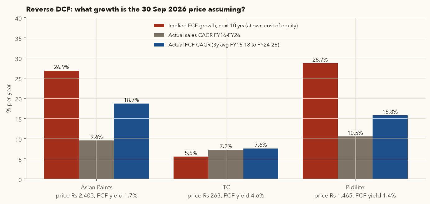
| 30 Sep 2026 | FCF yield | Implied g @ own \(K_e\) | Implied g @ 12% | Sales CAGR FY16–26 | Implied return if FCF grows like sales |
|---|---|---|---|---|---|
| Asian Paints | 1.72% | 26.9% | 23.4% | 9.6% | 7.4% |
| Pidilite | 1.40% | 28.7% | 26.1% | 10.5% | 7.1% |
| ITC | 4.63% | 5.5% | 8.3% | 7.2% | 11.1% |
It inherits every DCF weakness: the base FCF, the terminal growth and the discount rate are still your choices. Its real strength is psychological. It replaces "what is this worth?", which invites optimism, with "what has to go right?", which invites skepticism. If the answer is "growth no Indian consumer company has sustained for a decade", you have learned something important.
11. Dividend discount model (ITC)
For a mature company that pays out most of its earnings, the cash shareholders actually receive is the dividend. The dividend discount model (DDM) values the share as the PV of all future dividends. With constant growth it reduces to the Gordon formula:
- \(P_0\)
- The value of one share today (the subscript 0 means "now"), in ₹. In the second formula it is today's market price.
- \(D_0\)
- The dividend per share paid over the last year, in ₹.
- \(D_1\)
- The dividend per share expected over the next year, in ₹. \(D_1 = D_0 \times (1+g)\).
- \(K_e\)
- Cost of equity from CAPM (Section 6), as a decimal.
- \(g\)
- The yearly growth rate of the dividend, assumed to last forever. Must be below \(K_e\).
- \(g_{implied}\)
- The forever growth rate that today's price is assuming.
- \(\Longleftrightarrow\)
- "Is equivalent to": the right-hand formula is the left-hand one rearranged.
How it works: it is the same perpetuity idea as the terminal value in Section 7, applied to dividends. Next year's dividend divided by the gap \(K_e - g\) gives the value of all future dividends. Turn it around, plug in today's price, and you get the growth rate the market is assuming.
Valuing ITC on its dividends
- FY26 EPS = ₹16.51, payout ratio 88%, so \(D_0\) ≈ 16.51 × 0.88 = ₹14.53. (Dividends actually paid in the 12 months to 30 Sep 2026 per our price file: ₹14.50.) Dividend yield = 14.53 / 262.75 = 5.53%.
- \(K_e\) = 10.75% (from CAPM above).
- At g = 5%: \(D_1\) = 14.53 × 1.05 = 15.26, and \(P_0 = 15.26/(0.1075 - 0.05) = \mathbf{₹265.3}\). The market price is ₹262.75.
- At g = 4%: ₹223.9. At g = 6%: ₹324.2. A one-point change in growth moves value by about ±20%.
- Implied growth at today's price: \((0.1075 \times 262.75 - 14.53)/(262.75 + 14.53) = \mathbf{4.95\%}\).
The DDM and the FCF reverse DCF agree: the market is pricing ITC for roughly 5% long-run growth.
DDM is useless for companies that pay little or no dividend but reinvest heavily (DMart, Trent, Titan), because their value comes from reinvestment, not payouts. It also breaks when payout ratios change a lot. Use it for high-payout, slow-growth businesses: ITC, Coal India, some PSUs and utilities. Varsity's core modules focus on DCF for this reason.
12. Relative valuation: P/E, P/S, P/B, EV/EBITDA, PEG
Multiples are shortcuts: price divided by some measure of what you get. They are quick and they reflect market reality, but they hide the assumptions a DCF makes explicit. Use them to compare like with like: a company with its own history, or with close peers.
12.1 Price to earnings (P/E)
- Price per share
- Today's share price, in ₹.
- EPS
- Earnings per share: net profit for a year ÷ number of shares, in ₹. Trailing (TTM) EPS uses the last four quarters.
- Market cap
- Price × shares outstanding, in ₹ crore.
- Net profit
- Profit after tax for the same 12 months, in ₹ crore.
- Earnings yield
- Profit as a % of the price you pay: the P/E turned upside down.
How it works: dividing per share or for the whole company gives the same answer, because the number of shares cancels out. Earnings yield flips the ratio so you can compare it with an interest rate.
Example (Pidilite, 30 Sep 2026, table below): \(1{,}465.1 / 26.02 = 56.3\). Earnings yield \(= 1/56.3 = 1.78\%\), against a 7.18% G-sec yield.
P/E is how many rupees investors pay today for one rupee of annual profit. Its inverse, the earnings yield, lets you compare a stock with a bond. A P/E of 20 is an earnings yield of 5%. A trailing P/E uses the last 12 months' EPS (TTM). A forward P/E uses next year's estimate, which is more relevant but is someone's guess.
Why P/Es differ (the logic): from the Gordon model, a "fair" P/E ≈ payout × (1 + g)/(\(K_e\) − g). P/E rises with growth and with the quality (sustainability) of growth, and falls with risk and with interest rates. A high P/E is not "bad". It is a bet that growth will be high and long-lasting.
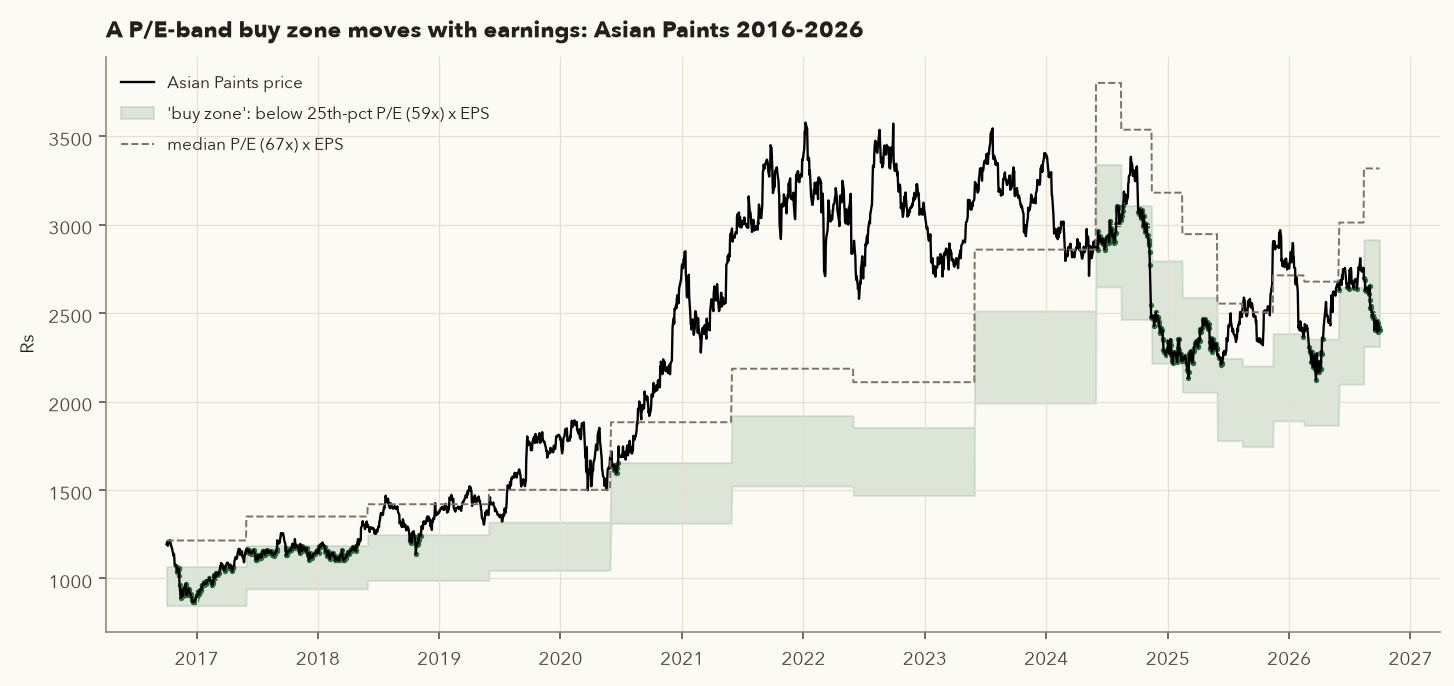
P/E band chart. Plot price alongside lines of EPS × fixed multiples. You immediately see whether the stock is trading at the top or bottom of its historical range.
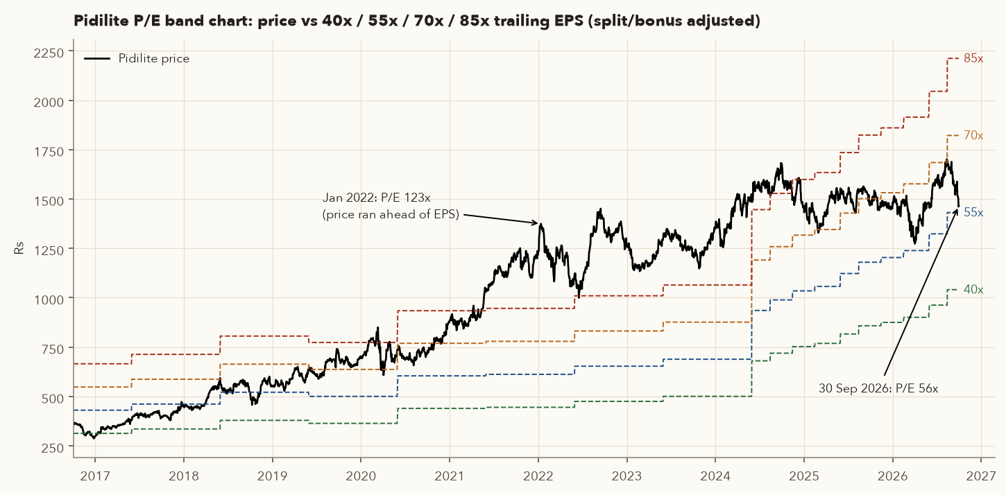
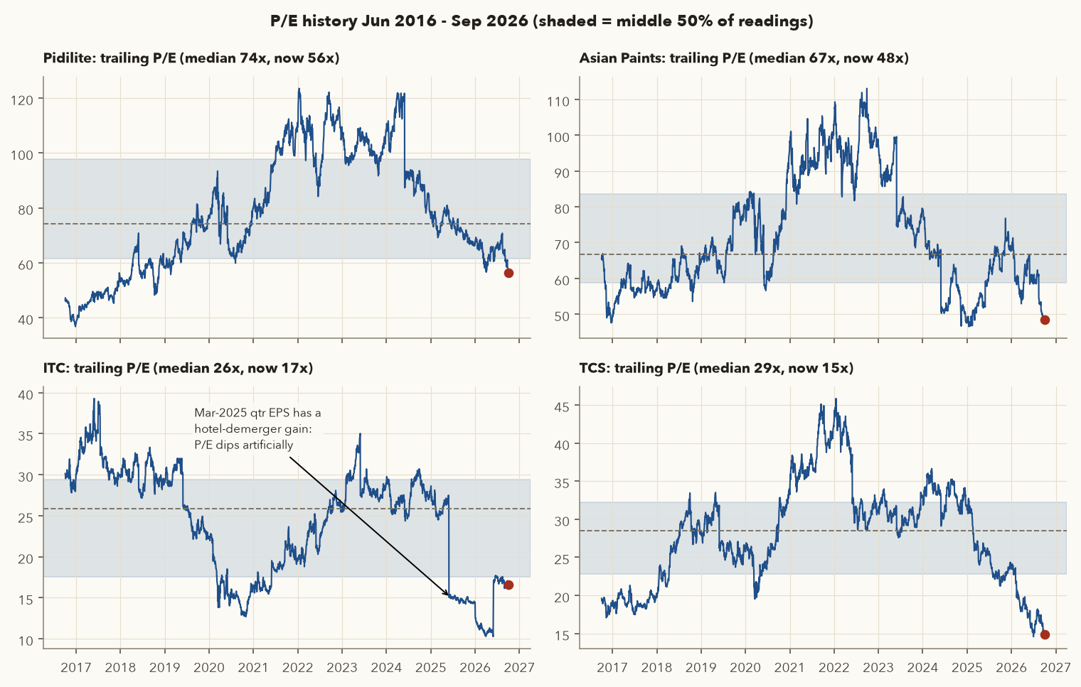
| 30 Sep 2026 | Price ₹ | TTM EPS ₹ | P/E now | 10y median P/E | 10y 25th pct | 10y range |
|---|---|---|---|---|---|---|
| Pidilite | 1,465.1 | 26.02 | 56.3 | 74.2 | 61.4 | 36.7–123.5 |
| Asian Paints | 2,402.6 | 49.68 | 48.4 | 66.8 | 58.7 | 46.5–113.0 |
| ITC | 262.75 | 15.84 | 16.6 | 25.9 | 17.6 | 10.3–39.3 |
| TCS | 2,050.6 | 137.64 | 14.9 | 28.5 | 22.8 | 14.6–45.8 |
| Titan | 4,587.0 | 64.89 | 70.7 | 85.9 | 74.0 | 39.9–247.5 |
| DMart | 3,801.4 | 46.94 | 81.0 | 121.4 | 102.1 | 78.4–313.7 |
| HDFC Bank | 708.7 | 51.35 | 13.8 | 23.9 | 20.0 | 13.4–34.3 |
Varsity's personal rule of thumb is to avoid stocks above 25–30x earnings. Today's Indian market routinely pays more for consumer franchises. Treat such rules as starting points, and always ask what growth the multiple implies (section 10).
12.2 Price to sales (P/S)
- Market cap
- Price × shares outstanding, in ₹ crore.
- Sales
- Revenue for the last 12 months (TTM), in ₹ crore.
How it works: it tells you how many rupees investors pay for each rupee of yearly sales. Because sales are rarely negative, it still works when profits are tiny or losses. But a rupee of sales is worth more when more of it turns into profit, so read it next to the net margin.
Useful when earnings are temporarily depressed or negative, for example a cyclical at the bottom or a young company. Always read it next to the profit margin. Pidilite trades at 1,48,628 / 15,399 TTM sales = 9.65x sales with a 17.4% net margin. Asian Paints trades at 2,29,440 / 37,187 = 6.17x sales with a 13.0% net margin. A rupee of Pidilite's sales carries more profit, which partly explains the higher P/S.
12.3 Price to book (P/B), the right lens for banks
- Price
- Today's share price, in ₹.
- Book value per share
- (BVPS) Shareholders' equity on the balance sheet ÷ number of shares, in ₹.
- ROE
- Return on equity: net profit ÷ average shareholders' equity (chapter 7), in %. The long-run level you expect the bank to sustain.
- \(g\)
- Long-run yearly growth rate of earnings and book value, in %.
- \(K_e\)
- Cost of equity from CAPM (Section 6), in %.
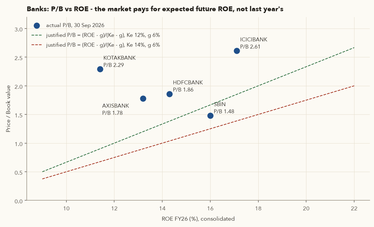
How it works: the first ratio is what the market pays per rupee of book value. The second is what it should pay given the bank's returns. A bank earning exactly its cost of equity (ROE = \(K_e\)) makes the top and bottom equal, so it is worth exactly book (P/B = 1). Earn more and it deserves a premium, earn less and it deserves a discount.
A bank's assets (loans) and liabilities (deposits) are financial and carried close to their real value, so book value means something. Its "raw material" is money, which makes EV and FCF awkward. For manufacturing or consumer businesses whose value lies in brands and know-how, P/B means little.
Is HDFC Bank's P/B justified by its ROE?
- Book value FY26 = ₹5,86,059 cr; shares 1,540.11 cr; BVPS = ₹380.5. P/B = 708.7/380.5 = 1.86.
- ROE = FY26 profit 79,219 / average equity (5,21,789 + 5,86,059)/2 = 14.3%.
- \(K_e\) = 7.18% + 0.97 × 7% = 13.97%. Assume long-run g = 6%.
- Justified P/B = (14.3% − 6%) / (13.97% − 6%) = 1.04, well below the actual 1.86.
- Reverse it: to justify 1.86 at a 13.97% cost of equity, sustainable ROE would need to be about 20.9%. Or, at a 14.3% ROE, investors must be using a cost of equity of only about 10.5%.
The market is betting on higher future ROE than FY26's (the post-merger dip), or it treats HDFC Bank as lower-risk than CAPM suggests. Both are judgements you have to make.
Why chapter 7 shows slightly different numbers (P/B 1.94, ROE 14.0%): it uses the standalone bank. Here we use consolidated figures, because the share price also pays for the subsidiaries (HDB Financial, HDFC Life, HDFC AMC and others). Both are fine as long as price, book value and profit come from the same basis.
12.4 EV/EBITDA
- EV
- Enterprise value: the market value of the whole business, shareholders' part plus net debt, in ₹ crore.
- Market cap
- Price × shares outstanding, in ₹ crore.
- Debt
- Total borrowings, in ₹ crore.
- Cash
- Cash and equivalents, in ₹ crore.
- EBITDA
- Earnings before interest, tax, depreciation and amortisation for the last 12 months (TTM), in ₹ crore: operating profit before any charges for debt or fixed assets.
How it works: first build EV: what you would pay for all the shares, plus the debt you would take on, minus the cash you would get. Then divide by EBITDA. The answer is how many years of current operating profit the whole business costs.
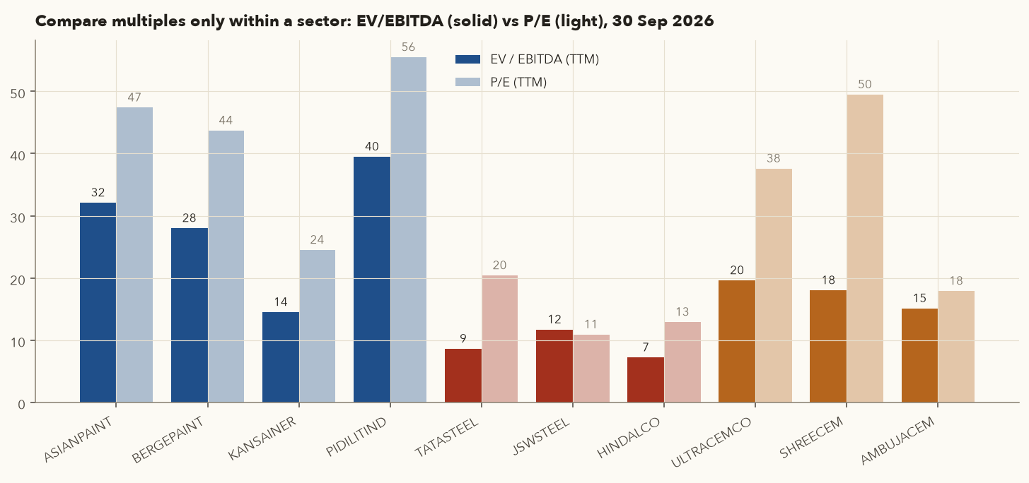
EV/EBITDA is capital-structure neutral. EV includes debt and EBITDA is before interest, so a heavily indebted company and a debt-free one can be compared fairly. It also ignores depreciation policies. That makes it the standard multiple for capital-heavy, leveraged sectors: steel, cement, telecom, power, infrastructure. Its blind spot is that EBITDA ignores capex, which in these sectors is huge and very real.
Why P/E and EV/EBITDA disagree for a leveraged company
- Market cap ₹2,29,636 cr + borrowings ₹92,382 cr − cash ₹10,058 cr = EV ₹3,11,960 cr.
- TTM EBITDA ₹36,189 cr. EV/EBITDA = 8.6x.
- P/E = market cap ÷ TTM consolidated net profit (₹11,263 cr) = 20.4x. On TTM EPS attributable to Tata Steel's own shareholders (₹8.83, which excludes the minority share), price ÷ EPS = 20.9x. Either way, interest (₹7,085 cr TTM) and heavy depreciation (₹12,850 cr TTM) eat most of the EBITDA before it reaches shareholders, so P/E looks "expensive" while EV/EBITDA looks moderate. Compare steel with steel on EV/EBITDA, and note net debt/EBITDA (2.27x here) as a risk measure.
12.5 PEG ratio
- \(P/E\)
- The price-to-earnings ratio from 12.1 (here, trailing 12 months).
- EPS growth rate
- Yearly growth in earnings per share, entered as a plain number of percent (11.3% is entered as 11.3, not 0.113). The table below uses the 5-year CAGR from FY21 to FY26.
How it works: divide the P/E by the growth rate to see how much you pay per point of growth. A PEG near 1 means the P/E roughly matches the growth rate. The result is only as good as the growth number you put in.
Example (TCS, table below): P/E 14.9, EPS growth 9.2% a year, so PEG = 14.9 / 9.2 = 1.62.
PEG adjusts P/E for growth. A popular rule of thumb (from Peter Lynch) says PEG ≈ 1 is fair and below 1 is attractive. The catch is that the growth used must be sustainable future growth, and past growth can be badly distorted:
| 30 Sep 2026 | TTM P/E | EPS FY21 | EPS FY26 | 5y EPS CAGR | PEG | Caution |
|---|---|---|---|---|---|---|
| HDFC Bank | 13.8 | 28.87 | 49.39 | 11.3% | 1.22 | Bank: also read P/B, ROE |
| TCS | 14.9 | 87.67 | 136.01 | 9.2% | 1.62 | Past growth may not repeat |
| Titan | 70.7 | 10.96 | 57.14 | 39.1% | 1.81 | FY21 was a COVID-hit base: growth flattered |
| ITC | 16.6 | 10.69 | 16.51 | 9.1% | 1.83 | FY21 was a COVID-hit base; the hotels business was demerged in Jan 2025, so FY26 EPS excludes it |
| Pidilite | 56.3 | 11.13 | 24.06 | 16.7% | 3.38 | |
| DMart | 81.0 | 16.97 | 45.56 | 21.8% | 3.71 | |
| Asian Paints | 48.4 | 32.73 | 45.09 | 6.6% | 7.31 | Earnings dipped in FY25 |
| Trent | 77.3 | −2.74 | 32.25 | n/m | n/m | Loss-making base: PEG undefined |
12.6 Which multiple when?
| Business type | Primary multiple(s) | Avoid / be careful with |
|---|---|---|
| Steady consumer, IT services, pharma | P/E (vs own history and peers), PEG, DCF/reverse DCF | P/B (brands are not on the balance sheet) |
| Banks, NBFCs, insurers | P/B with ROE, P/E | EV/EBITDA, FCF-based DCF |
| Cyclicals: metals, cement, chemicals, autos | EV/EBITDA on mid-cycle EBITDA, P/B at troughs | P/E at peak earnings (section 13) |
| Capital-heavy and leveraged: telecom, power, infra | EV/EBITDA, net debt/EBITDA | P/E (distorted by interest and depreciation) |
| High-payout, slow growth: ITC, utilities, PSUs | Dividend yield, DDM, FCF yield | PEG (growth too low to be meaningful) |
| Loss-making or early-stage | P/S (with a path to margins), scenario DCF | P/E, PEG (undefined) |
13. Valuation pitfalls, with real failures
13.1 Garbage in, garbage out
A DCF has no opinion of its own. It multiplies whatever you feed it. Our Pidilite value moves from ₹326 to ₹705 just by changing stage-1 growth from 8% to 20%. Defend each input with history, industry context and management commentary. Write your reasons down (Varsity suggests a "working notes" sheet), and update the model when facts change, not when the price changes.
13.2 Terminal value dominance
In our base case 53% of Pidilite's value comes from cash flows after 2036, and with an exit multiple it is 76%. If most of your answer depends on what happens more than 10 years away, be humble about precision and generous with margin of safety.
13.3 Cyclicals: the low P/E trap
For commodity businesses, earnings swing far more than the business's long-term value. At the top of the cycle, earnings are huge and P/E looks tiny. At the bottom, earnings collapse and P/E looks enormous. Reading those P/Es naively gets you exactly backwards.
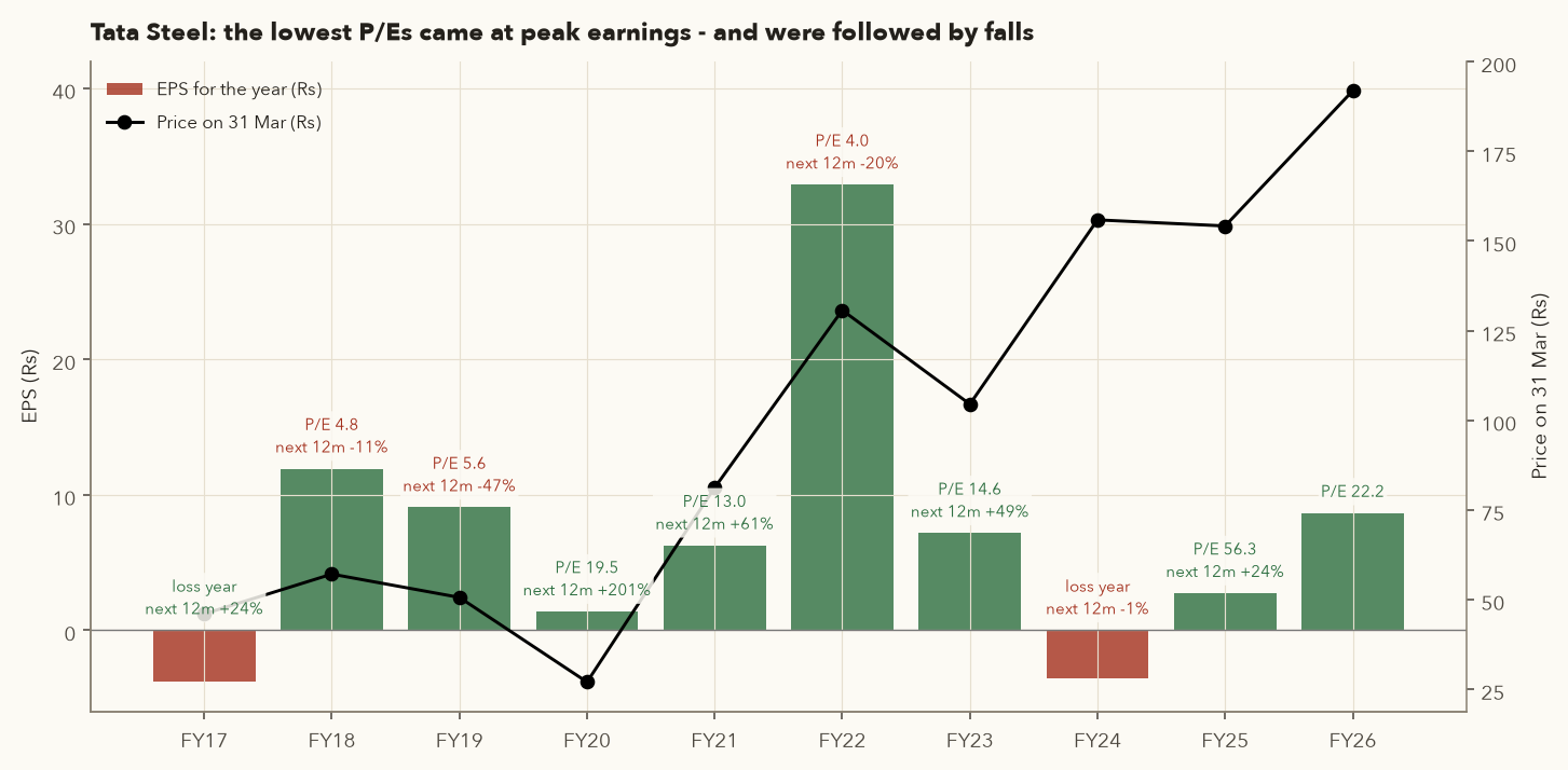
| 31 Mar | EPS for the year ₹ | Price ₹ | P/E | Next 12 months |
|---|---|---|---|---|
| 2018 | 11.93 | 57.1 | 4.8 | −11.3% |
| 2019 | 9.07 | 50.6 | 5.6 | −46.8% |
| 2020 | 1.38 | 27.0 | 19.5 | +201.1% |
| 2021 | 6.26 | 81.2 | 13.0 | +61.0% |
| 2022 | 32.88 | 130.7 | 4.0 | −20.1% |
| 2023 | 7.17 | 104.5 | 14.6 | +49.1% |
| 2024 | −3.55 | 155.9 | loss | −1.0% |
| 2025 | 2.74 | 154.2 | 56.3 | +24.4% |
| 2026 | 8.65 | 191.9 | 22.2 | — |
The three lowest P/Es (4.0, 4.8, 5.6) were all followed by price falls. The highest (19.5 in March 2020 on collapsed earnings, and 56.3 in 2025) were followed by gains of 201% and 24%. FY22 EPS of ₹32.88 was a peak: it fell to ₹7.17 the next year and to a loss the year after. For cyclicals, value the business on normalised (mid-cycle) earnings, or use EV/EBITDA on average-cycle EBITDA and P/B, never on peak P/E. Note that these P/Es use each year's full EPS, which the market only learned after the year ended, so they flatter the "low P/E" signal. In real time it would have looked even more convincing, and been even more wrong.
13.4 One-off gains distort P/E
The "cheap" P/E that wasn't
- Hindustan Unilever's TTM EPS on 30 Sep 2026 is ₹63.66, giving a P/E of just 29.5 against a 10-year median of about 64.
- But the Dec-2025 quarter shows EPS of ₹28.12 with other income of ₹4,048 cr. The other three quarters earned ₹11.38–₹12.73 with other income of ₹113–₹503 cr. A one-off gain sits in that quarter.
- Replace the Dec-2025 quarter with the average of the other three and normalised EPS = ₹47.39. The P/E becomes 39.7, much closer to screener.in's own figure.
- ITC had the same issue: its Mar-2025 quarter EPS of ₹15.76 (vs about ₹4 normally) included a gain linked to the hotels demerger. That is why its P/E chart dips to 10–15x from mid-2025 to mid-2026 (figure in 12.1).
Rule: before trusting any P/E, scan the last four quarters for jumps in "other income" or "exceptional items" (chapter 6).
13.5 Negative or tiny free cash flow: DCF does not fit
DMart's three-year average CFO − capex is −₹525 cr, because it keeps buying land and building stores. Titan's FCF yield is only 0.39%, because gold inventory absorbs cash as it grows. A mechanical DCF values both near zero or below. That says nothing useful about their worth: their value is in the returns on reinvestment. For such businesses, model a future steady state (when capex slows) or use P/E and ROCE-based reasoning instead.
13.6 Look-ahead bias: the buy zone that only worked in hindsight
Here is a tempting rule: "buy when P/E is below its 10-year 25th percentile." On Asian Paints, using the full 2016–2026 history to set the threshold (59x), the median 1-year return after an in-zone day was +15.7% vs +8.6% otherwise. Great?
No. That threshold used the future. Redo it honestly: each day, use only the trailing 5 years of P/E to set the 25th-percentile threshold (testable from Oct 2018):
| Real-time rule, Oct 2018 – Sep 2025 start dates | Days in zone | Median 1-yr return in zone | Median 1-yr return otherwise | % of in-zone days with a loss |
|---|---|---|---|---|
| Asian Paints | 400 | −6.5% | +11.6% | 56% |
| Pidilite | 204 | +2.1% | +15.9% | 41% |
| ITC | 654 | −4.5% | +7.0% | 52% |
| TCS | 156 | −30.4% | +8.6% | 100% |
In real time, "below its usual P/E" was followed by worse returns for all four. De-ratings tend to persist: a P/E usually falls because the outlook changed, and it can keep falling. This does not mean P/E bands are useless. It means a low P/E is a reason to research, not a reason to buy, and that any rule you test must use only information available at the time. Chapter 12 covers backtesting discipline in depth.
13.7 Value traps and changed regimes
Earnings up, price down by half
- 30 Sep 2024: TCS closed at ₹4,268.5 on trailing EPS of ₹129.21, a P/E of 33.0.
- 30 Sep 2026: ₹2,050.6 on EPS of ₹137.64, a P/E of 14.9.
- EPS rose 6.5% while the price fell 52.0%. The whole loss came from the multiple.
The market re-rated the entire business: slower growth, new competitive threats, a changed view of what IT services will earn. A 10-year P/E median of 28.5 is meaningless if the next 10 years look different. A stock that keeps getting "cheaper" because its prospects keep shrinking is a value trap. Reverse DCF helps here: at ₹2,050.6, TCS's 6.05% FCF yield implies only 5.7% a year FCF growth at a 12% discount rate. The question is whether even that is achievable, and a P/E chart cannot answer it.
13.8 Other common mistakes
- Mixing adjusted and unadjusted data. Splits and bonuses (Pidilite 1:1 in 2025, HDFC Bank 1:1 in 2025) change the share count. Use EPS and prices on the same basis.
- Standalone vs consolidated. Use consolidated numbers for groups with subsidiaries. For banks with big subsidiaries (HDFC Bank, Kotak, ICICI), value the subsidiaries separately ("sum of the parts") if you want precision.
- Forgetting dilution: ESOPs, warrants and planned equity raises.
- Discounting nominal cash flows at a real rate (or the reverse). Keep everything in nominal rupees.
- Precision theatre. "Fair value ₹1,237.45" signals false confidence. Say "roughly ₹1,100–1,350".
14. Valuing the whole market: Nifty P/E and bond yields
An index has a P/E too: NSE divides the combined free-float market cap of the 50 stocks by their combined earnings and publishes the Nifty's P/E, P/B and dividend yield daily (Varsity: NSE website → indices → historical P/E, P/B & dividend yield).
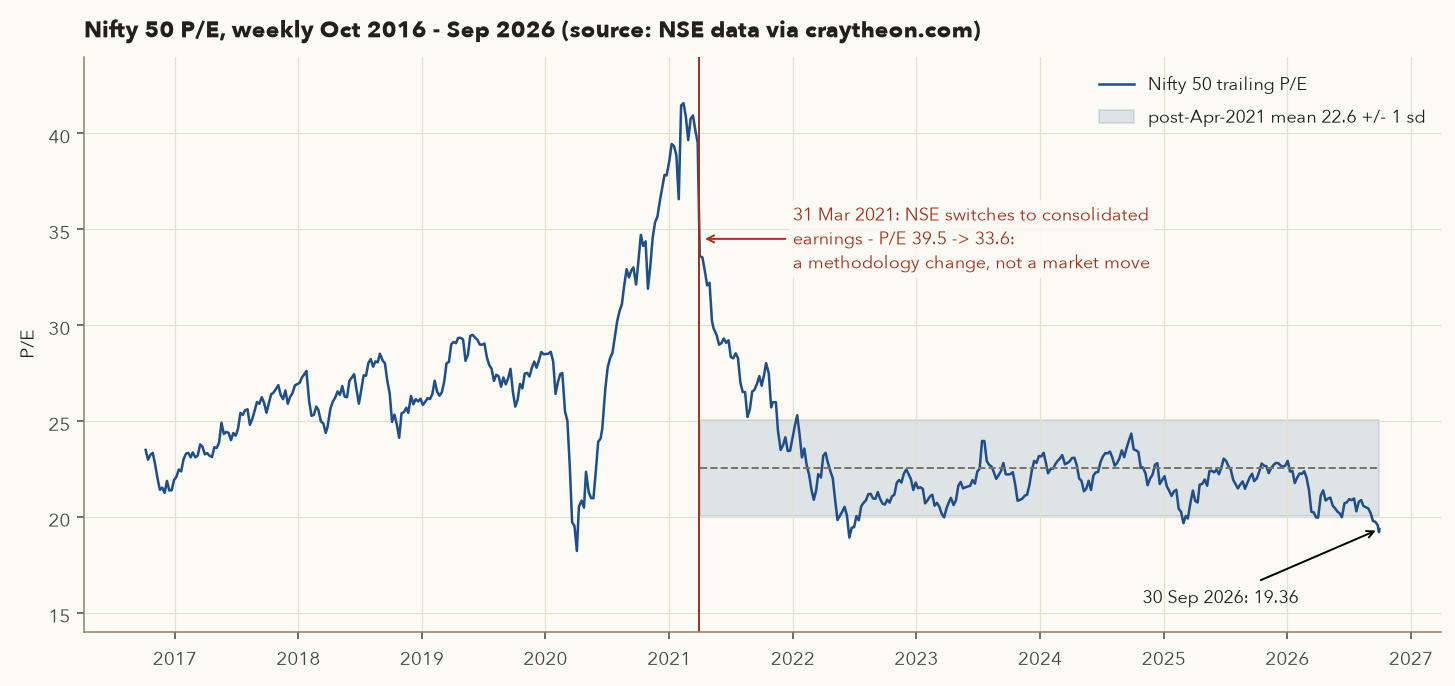
On 31 Mar 2021 NSE switched the index P/E from standalone to consolidated earnings. Consolidated profits are larger, so the P/E dropped overnight (39.51 to 33.60 in our weekly data) with no change in price. Varsity's well-known guide, written in 2014 on standalone data ("cautious above 22x, attractive at 16x or below"), cannot be applied directly to today's numbers. Use only the post-April-2021 history for comparison.
Where the market stands (post-Apr-2021 consolidated series): mean 22.57, standard deviation 2.50, range 18.92–33.60. At 19.36 on 30 Sep 2026, only about 1% of weekly readings since April 2021 were lower. A year earlier the P/E was 21.86. The Nifty fell 8.1% over the year (24,611.1 → 22,620.45). The P/E implies trailing Nifty EPS of about 22,620.45 / 19.36 ≈ 1,168.
Earnings yield vs bond yield
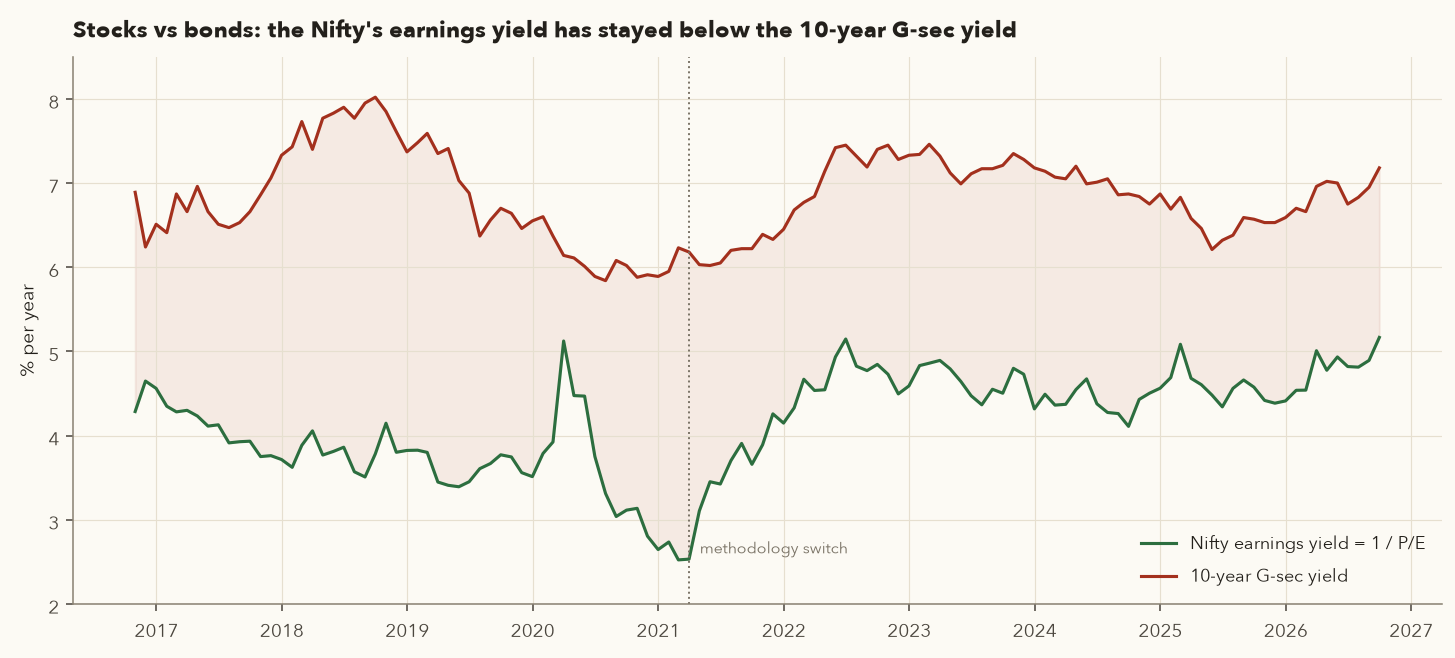
Compare what stocks "earn" on their price with what a risk-free bond pays. The yield gap = earnings yield − G-sec yield. The bond-equity earnings yield ratio (BEER) = G-sec yield ÷ earnings yield.
Stocks vs bonds today
- Earnings yield = 1 / 19.36 = 5.17%. G-sec = 7.18%.
- Yield gap = 5.17% − 7.18% = −2.01 points. BEER = 7.18 / 5.17 = 1.39.
- Since April 2021 the monthly gap averaged −2.36 points, ranging from −2.93 (Apr 2021, expensive stocks) to −1.73 (May 2025). Today is on the "less expensive than usual" side of that range.
Indian equities almost always yield less than bonds on current earnings, because investors expect earnings to grow and bond coupons do not. The change in the gap is more informative than its level.
Does a low market P/E predict higher returns?
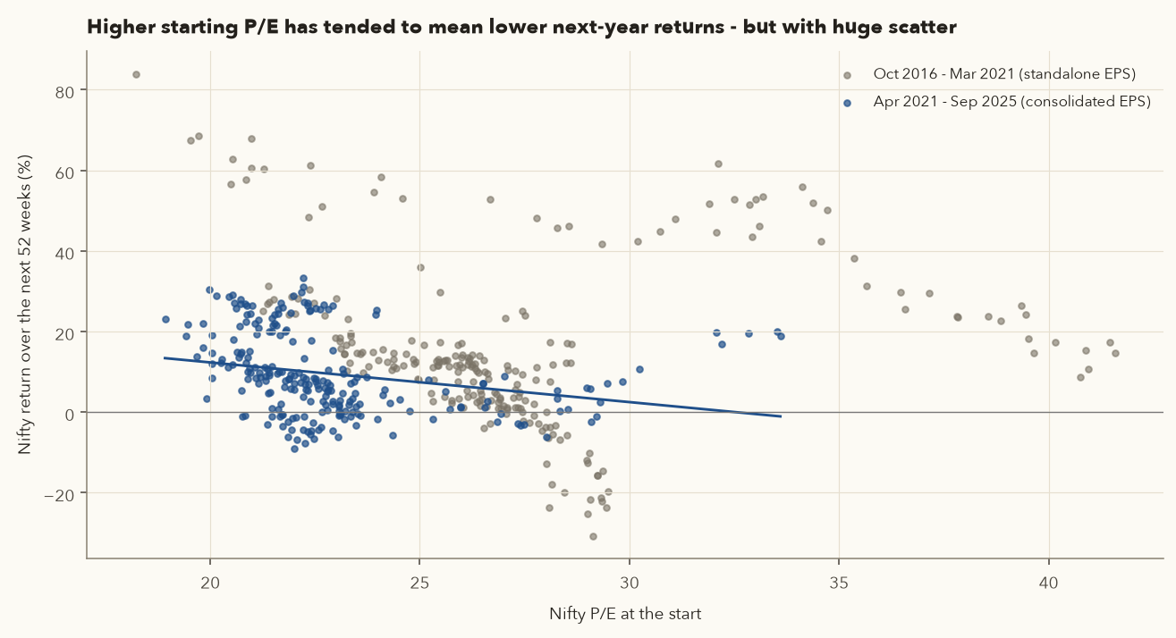
| Starting P/E (post-Apr-2021, weekly) | Weeks | Median next-52-week return | % of weeks with a loss |
|---|---|---|---|
| Below 21 | 45 | +15.2% | 4% |
| 21–23 | 120 | +8.0% | 21% |
| 23–25 | 37 | +1.8% | 30% |
| Above 25 | 34 | +3.0% | 26% |
Post-2021 the correlation between starting P/E and next-year return is −0.25: a modest tendency, with huge scatter. In 2016–2021 it was only −0.06, because 2020's collapsed earnings made the P/E spike just before a huge rally (the same cyclical trap as Tata Steel, at index level). With only about five years of comparable data and overlapping windows, treat this as context, not a timing tool. A low index P/E improves your odds over years. It does not tell you next month's direction, so swing traders should still trade price (chapters 3–5).
15. Building a watchlist with buy-zone prices
Valuation pays off when you prepare. Decide in advance, calmly, what you would pay for businesses you like. When the market offers that price (often in a panic), you act on a plan instead of a feeling. Varsity notes that long-term opportunities "linger": a stock can sit in a value zone for months, so there is no need to rush.
A simple two-lens process
- Quality gate first (chapter 7): only businesses with consistent ROCE, cash conversion and clean governance get on the list.
- Lens 1, own history: P/E buy level = 25th-percentile P/E (10 years) × TTM EPS. It tells you when the stock is cheap relative to how the market usually values it.
- Lens 2, cash flows: reverse DCF at a fixed 12% discount rate and 5% terminal growth. Compare the implied growth with the better of the 5-year EPS CAGR and the 10-year sales CAGR. It tells you whether the price needs heroics.
- Optional DCF value: stage-1 growth = 10-year sales CAGR (capped at 15%), stage 2 = two-thirds of that (at least 5%), terminal 5%, discount 12%. Then apply a 25% margin of safety.
- Classify: both lenses favourable means research in depth; only one means keep watching; neither means move on. Re-run quarterly after results.
| 30 Sep 2026 | Price | P/E now | P/E buy level (25th pct × EPS) | Implied FCF g @12% | Hist. growth (max of EPS 5y, sales 10y) | DCF @12% / with 25% MOS | Classification by the rule |
|---|---|---|---|---|---|---|---|
| Pidilite | 1,465.1 | 56.3 | 1,598 | 26.1% | 16.7% | 454 / 341 | Cheap vs own history; price still needs above-history growth |
| Asian Paints | 2,402.6 | 48.4 | 2,916 | 23.4% | 9.6% | 825 / 619 | Cheap vs own history; price still needs above-history growth |
| ITC | 262.75 | 16.6 | 279 | 8.3% | 9.1% | 232 / 174 | Both lenses favourable: research in depth |
| TCS | 2,050.6 | 14.9 | 3,138 | 5.7% | 9.4% | 2,423 / 1,817 | Both lenses favourable: research in depth (but see 13.7) |
| Titan | 4,587.0 | 70.7 | 4,802 | n/m | 39.1% | n/m | FCF yield 0.39%: DCF not meaningful, P/E lens only |
| DMart | 3,801.4 | 81.0 | 4,793 | n/m | 23.1% | n/m | Negative FCF: DCF not meaningful, P/E lens only |
Source: author's calculations (script course/scripts/ch08_figures.py). The classification is the mechanical output of the rule above, shown to illustrate the method. It is not a recommendation.
How to read this honestly:
- All six stocks are below their own P/E buy level. That says more about the 2025–26 de-rating of quality stocks than about bargains. Section 13.6 showed that buying on this lens alone, in real time, has done badly.
- The cash-flow lens separates them. Pidilite and Asian Paints still need roughly 23–26% a year FCF growth at a 12% discount rate. ITC and TCS need less than they have historically delivered.
- "Research in depth" means read the annual report, the last few concall transcripts and the risks. For TCS, ask whether the drop reflects a temporary scare or a permanent change (13.7). For ITC, weigh regulatory and tax risk on cigarettes.
- Even then, phase your buying (for example in three tranches over a few months) and size positions with risk rules (chapter 11). Valuation tells you what is reasonable to buy. It never tells you when the price will turn.
Varsity's closing chapter on fundamentals gives three good reasons to exit a long-term holding. Write them down next to your buy level:
- The thesis broke. The reason you bought (margins, market share, management quality, balance-sheet strength) no longer holds. A quarter or two of weak numbers is not enough; a lasting change in the business is.
- The price ran far ahead of value. Your reverse DCF now needs growth the business has never delivered, the way Asian Paints did at 109x in January 2022 (section 2). You can trim instead of selling everything.
- A clearly better use of the money. Another business on your watchlist offers similar quality with much more margin of safety.
A falling price on its own is not on this list. If the thesis holds and value has not changed, a lower price only improves the margin of safety. That is where position sizing and the risk limits of chapter 11 come in: they keep you able to hold, or add, through a drawdown.
Keep a spreadsheet or a Python dict per stock: quality score, buy level, fair value range, implied growth, your thesis in two lines, what would make you sell. Update after each quarterly result. In chapter 17 you will wire framework.fundamentals.quality_scorecard, dcf and reverse_dcf into a single python -m framework.invest SYMBOL report, and combine it with chart-based entries from chapters 3–5.
16. Try it yourself (Python)
These snippets need a copy of the course repository and Python with pandas and numpy (setup steps are in its framework/README.md). Run them from the repository's root folder, for example with .venv/bin/python, because the file paths are relative to that folder. Each reproduces a number from this chapter using the course data. The full analysis, every figure and every number is in course/scripts/ch08_figures.py, which writes all values to data/extra/ch08_numbers.json.
1. Beta and cost of equity
import pandas as pd, numpy as np
D = "data/ohlc/"
stock = pd.read_csv(D + "PIDILITIND.csv", index_col=0, parse_dates=True)["Adj Close"]
nifty = pd.read_csv(D + "IDX_NSEI.csv", index_col=0, parse_dates=True)["Close"]
df = pd.concat([stock, nifty], axis=1, keys=["s", "m"], sort=True).loc["2023-09-30":"2026-09-30"].dropna()
w = df.resample("W-FRI").last().pct_change().dropna()        # weekly returns
beta = np.cov(w.s, w.m)[0, 1] / w.m.var()
rf, erp = 0.0718, 0.07
print(f"weeks={len(w)}  beta={beta:.2f}  cost of equity={rf + round(beta, 2) * erp:.2%}")
# -> weeks=156  beta=0.84  cost of equity=13.06%
2. A DCF with a sensitivity grid
def dcf(fcf0, growth, r, g, net_cash, shares):
    """growth = list of yearly growth rates; returns (value per share, TV share of EV)."""
    pv, fcf = 0.0, fcf0
    for t, gt in enumerate(growth, start=1):
        fcf *= 1 + gt
        pv += fcf / (1 + r) ** t
    tv = fcf * (1 + g) / (r - g)                 # Gordon growth terminal value at year N
    pv_tv = tv / (1 + r) ** len(growth)
    ev = pv + pv_tv
    return (ev + net_cash) / shares, pv_tv / ev

# Pidilite, Rs crore: 3-yr avg FCFF, 12% x5 then 9% x5, WACC 13%, g 5%
value, tv_share = dcf(1943.5, [0.12] * 5 + [0.09] * 5, 0.13, 0.05, net_cash=299 + 4350 - 417, shares=101.45)
print(f"value/share Rs {value:.0f}, terminal value = {tv_share:.0%} of EV")   # Rs 418, 53%

for r in [0.11, 0.12, 0.13, 0.14, 0.15]:          # sensitivity row by row (g = 4%, 5%, 6%)
    print(f"WACC {r:.0%}:", [round(dcf(1943.5, [0.12]*5 + [0.09]*5, r, g, 4232, 101.45)[0]) for g in (0.04, 0.05, 0.06)])
3. Reverse DCF (ITC)
from scipy.optimize import brentq

def equity_value(fcf0, g10, r, g_term, net_cash):
    pv, fcf = 0.0, fcf0
    for t in range(1, 11):
        fcf *= 1 + g10
        pv += fcf / (1 + r) ** t
    pv += fcf * (1 + g_term) / (r - g_term) / (1 + r) ** 10
    return pv + net_cash

fcf0, net_cash, mcap = 15193, 38738, 327863      # Rs crore, price Rs 262.75
for r in (0.10, 0.1075, 0.12):
    g = brentq(lambda x: equity_value(fcf0, x, r, 0.05, net_cash) - mcap, -0.3, 0.8)
    print(f"discount {r:.2%}: price implies {g:.1%} FCF growth for 10 years, then 5%")
# -> 3.7%, 5.5%, 8.3%
4. A simple P/E history (annual EPS only)
import pandas as pd
px = pd.read_csv("data/ohlc/ASIANPAINT.csv",
                 index_col=0, parse_dates=True)["Close"].loc["2016-06-01":]
eps_fy = {2016: 18.19, 2017: 20.22, 2018: 21.26, 2019: 22.48, 2020: 28.20, 2021: 32.73,
          2022: 31.59, 2023: 42.81, 2024: 56.92, 2025: 38.23, 2026: 45.09}   # screener.in, consolidated
eps = pd.Series({pd.Timestamp(f"{y}-05-31"): v for y, v in eps_fy.items()})  # known by end-May
eps = eps.reindex(px.index.union(eps.index)).ffill().reindex(px.index)
pe = px / eps
print(pe.describe().round(1))
print("25th pct P/E:", round(pe.quantile(.25), 1), "-> buy level on FY26 EPS:", round(pe.quantile(.25) * 45.09))
# median 66.8, 25th pct 58.5 -> 2,639. (The chapter uses quarterly TTM EPS from 2024, so its numbers differ slightly.)
5. Earnings yield vs G-sec
import pandas as pd
X = "data/extra/"
v = pd.read_csv(X + "ch08_nifty_pe_pb_dy_weekly_craytheon.csv", parse_dates=["Date"], index_col=0)
y = pd.read_csv(X + "ch08_india_10y_gsec_monthend_countryeconomy.csv", parse_dates=["Date"], index_col=0)
m = pd.concat([100 / v.pe.resample("ME").last(), y.Yield10y.resample("ME").last()], axis=1,
              keys=["earn_yield", "gsec"], sort=True).dropna()
m["gap"] = m.earn_yield - m.gsec
print(m.loc["2021-04":].describe().round(2))   # gap mean -2.36, range -2.93 to -1.73
print(m.tail(3).round(2))                      # Sep 2026: 5.17 vs 7.18, gap -2.01
Exercises with the code: (a) change Pidilite's WACC to 11% and stage-1 growth to 15% and see how far you get towards ₹1,465; (b) run the reverse DCF for Asian Paints (FCF 3,940, net cash 4,207, market cap 2,29,440); (c) compute beta over 5 years instead of 3 for ITC and see how \(K_e\) changes.
17. Practical checklist
- Has the business passed the quality checks (chapters 6–7) before I value it?
- Am I using consolidated numbers, adjusted for splits and bonuses, on the same basis as the price?
- Did I scan the last four quarters for one-off gains or losses before using TTM EPS?
- Base-year cash flow: did I average 3 years and check for working-capital swings and acquisitions?
- Discount rate: current 10-year G-sec yield (verified today), beta from my own data over 2–5 years, a stated ERP. Is WACC well above terminal growth?
- Growth: is each stage defended by history and industry context? Is terminal growth at most ~5–6%?
- What share of value comes from the terminal value? If over 60%, have I widened my margin of safety?
- Did I run a sensitivity grid (WACC × g, and stage-1 growth) and look at the whole range?
- Reverse DCF: what growth does today's price imply, and is it believable versus history?
- Is my multiple right for the business type (P/B for banks, EV/EBITDA for leveraged cyclicals, never peak P/E for cyclicals)?
- Am I comparing multiples within the same sector, or against the stock's own comparable history?
- Is this a de-rating that might continue (value trap)? What changed in the business?
- Index context: where is the Nifty P/E versus its post-2021 range, and the yield gap versus its range?
- Buy level and margin of safety written down before the price gets there; buying plan phased; position size set by risk rules.
- Thesis and "what would make me sell" written in two lines each; model updated after every quarterly result.
18. Key takeaways
- Price is what you pay; value is the present value of future cash. Asian Paints' EPS grew 42.7% from FY22 to FY26 while its price fell 32.8%, because the buyer in 2022 overpaid.
- Discounting turns future cash into today's value: \(PV = CF/(1+r)^t\). Higher rates and longer horizons shrink value fast.
- A DCF needs four things: a normal base-year free cash flow (FCFF), a growth path, a discount rate (CAPM for equity, WACC for the firm) and a terminal value. Then EV + net cash ÷ shares = value per share.
- Use current inputs: 10-year G-sec 7.18% (30 Sep 2026), ERP ~7% for India (Damodaran Jan 2026: 7.08%), beta from your own data.
- Our Pidilite base case gives ₹418 a share against a ₹1,465 price, and the terminal value is 53% of EV. The output is very sensitive to WACC, terminal growth and stage-1 growth, so think in ranges and demand a margin of safety.
- Reverse DCF asks what the price assumes. Asian Paints and Pidilite need about 26–29% a year FCF growth for a decade at their cost of equity; ITC needs about 5.5%. That is usually more useful than a point estimate.
- Match the multiple to the business: P/E and PEG for steady compounders, P/B with ROE for banks, EV/EBITDA for leveraged and capital-heavy firms, DDM or dividend yield for high-payout firms.
- Cyclicals look cheapest at peak earnings: Tata Steel's three lowest P/Es (4.0–5.6) were all followed by falls.
- Watch for one-offs (HUL's normalised P/E is 39.7, not 29.5), negative-FCF growers (DMart, Titan), look-ahead bias, and value traps (TCS: EPS +6.5%, price −52%).
- The Nifty's P/E of 19.36 is near the bottom of its post-2021 consolidated range (mean 22.57). Its 5.17% earnings yield is 2.01 points below the G-sec. That is context for years, not a timing signal.
- Build a watchlist with buy levels set in advance using more than one lens, then research, phase entries and size positions with risk rules.
19. Quiz and exercises
Q1. What is ₹50,000 receivable in 4 years worth today at 10%? And what does ₹50,000 invested today grow to in 4 years at 10%?
Q2. A company has EBIT ₹1,000 cr, tax rate 25%, depreciation ₹150 cr, capex ₹300 cr, and its working capital rose by ₹80 cr. Compute FCFF.
Q3. Using \(R_f\) = 7.18% and ERP = 7%, what is the cost of equity for a stock with β = 1.24 (Tata Steel)? Why can't you lower Tata Steel's WACC indefinitely by borrowing more?
Q4. A company's year-10 FCF is ₹500 cr. WACC 12%, terminal growth 5%. Compute the terminal value and its present value. Then recompute TV with g = 6%.
Q5. In our Pidilite DCF, enterprise value is ₹38,191 cr, cash ₹299 cr, investments ₹4,350 cr, borrowings ₹417 cr and shares 101.45 cr. Compute value per share and Varsity's ±10% band. With the price at ₹1,465.1, what would Varsity's rule say?
Q6. Asian Paints' reverse DCF implies 26.9% a year FCF growth for 10 years. Its sales grew 9.6% a year over FY16–26. What are three possible explanations, and what would you check?
Q7. ITC: \(D_0\) = ₹14.53, \(K_e\) = 10.75%, price ₹262.75. Find value at g = 5% and the implied g at today's price. When would DDM be a poor choice?
Q8. A bank has ROE 16%, cost of equity 13%, and long-run growth 6%. What P/B is justified? If it trades at 2.5x book, what ROE is the market implying?
Q9. Tata Steel traded at 4.0x FY22 EPS on 31 Mar 2022. Why was this not a bargain, and how should you value a cyclical instead?
Q10. HUL's TTM P/E is 29.5 versus a 10-year median of ~64. List the steps before concluding it is cheap.
Q11. Nifty P/E is 19.36 and the 10-year G-sec yields 7.18%. Compute the earnings yield, yield gap and BEER. Why can't you compare 19.36 with Varsity's 2014 thresholds of 16x and 22x?
Q12. A friend backtests "buy Pidilite when its P/E is below its 10-year 25th percentile" and reports excellent results. What is the flaw, and how do you fix the test?
20. Sources
Zerodha Varsity, Module 3, Fundamental Analysis: Ch. 11 The Financial Ratio Analysis (Part 3): valuation ratios and index valuation · Ch. 13 Equity Research (Part 1) · Ch. 14 DCF Primer · Ch. 15 Equity Research (Part 2): FCF, terminal value, NPV, share price, intrinsic value band · Ch. 16 The Finale: DCF limitations, margin of safety, when to sell.
Zerodha Varsity, Module 13, Integrated Financial Modelling: Ch. 14 Valuation Overview · Ch. 15 FCFF and FCFE · Ch. 16 Risk Premium and Tax Shield · Ch. 17 WACC and Terminal Growth · Ch. 18 Discounted Cash Flow Analysis. All concepts are explained in the course's own words.
Rates and premiums (checked Oct 2026): 10-year G-sec yield 7.18% on 30 Sep 2026, countryeconomy.com (month-end history saved to data/extra/ch08_india_10y_gsec_monthend_countryeconomy.csv); cross-check 7.16%, Trading Economics. Equity risk premium: Damodaran, Country Default Spreads and Risk Premiums (updated 5 Jan 2026): India total ERP 7.08%; Incwert, Assessment of India ERP, Jan 2026 (7.0%). Corporate tax 25.17% (section 115BAA of the 1961 Act; section 200 of the Income-tax Act, 2025 from tax year 2026-27): caclubindia (AY 2022-23 to 2026-27), TaxTMI, section (new) 200 / (old) 115BAA, incometaxindia.gov.in.
Nifty 50 P/E, P/B and dividend yield (weekly, Oct 2016 – Oct 2026): NSE index data as compiled by craytheon.com (saved to data/extra/ch08_nifty_pe_pb_dy_weekly_craytheon.csv); official source niftyindices.com historical P/E, P/B & Div. Yield. Switch to consolidated earnings on 31 Mar 2021: Upstox Learning Center.
Company financials: screener.in consolidated pages fetched 2 Oct 2026 (data/extra/screener_ch07/). Prices: NSE daily OHLC via Yahoo Finance to 30 Sep 2026 (data/ohlc/, data/extra/ch07_extra_closes_yf.csv). Calculations and figures: course/scripts/ch08_figures.py; all numbers in data/extra/ch08_numbers.json.