
Technical Indicators
1. What you'll learn and why it matters
In Chapters 2 and 3 you learned to read price itself: candles, support and resistance, trends and patterns. An indicator is a formula applied to that same price and volume data. It turns a messy chart into a cleaner number or line that answers one specific question: Is there a trend? How strong is it? Is the move overstretched? How big is a normal day's move?
By the end of this chapter you will be able to:
- Tell leading from lagging indicators, and oscillators from trend-following tools, and know what each family is good and bad at.
- Calculate by hand (and in Python) the SMA, EMA, RSI, MACD, Bollinger Bands, ATR, ADX/DMI, Supertrend, OBV, VWAP, Stochastic, Donchian channels and relative strength.
- Read the standard signals (crossovers, overbought/oversold, divergences, squeezes, band walks, breakouts), and recognise when each one usually fails.
- Use ATR to place stops and size positions, which is the single most practical use of any indicator in this chapter.
- Combine a small set of indicators that do different jobs (trend + momentum + volatility) rather than five that say the same thing.
Swing trader (days to weeks): you need a trend filter (moving averages, ADX), a timing tool (RSI, MACD, Bollinger) and a volatility tool (ATR) to set stops. Positional/long-term investor: the 50/200-day averages, weekly RSI and relative strength against Nifty help you avoid buying into falling knives and help you pick stocks that are already outperforming. Futures trader: leverage makes stop placement and position sizing non-negotiable, and ATR is the tool that tells you whether one lot is even affordable within your risk budget (Section 10 shows a real case where it is not).
On a first pass, focus on the core: Sections 2 (families), 3–5 (moving averages and trend filters), 6 (RSI), 10 (ATR for stops and sizing) and 18 (combining tools). Sections 7–9 and 11–15 each add one more tool; read them one at a time, ideally with the stock's chart open. Sections 16–17 are reference and evidence, and you can come back to them later.
No indicator predicts the future. Every one of them is a transformation of past prices, so it carries no information that was not already on the chart. They help you organise what you see and apply rules consistently. This chapter deliberately shows real cases where the textbook signal failed, along with a small statistical test across 37 stocks, so you build judgement rather than faith. All examples are historical analysis for education, not recommendations to buy or sell anything.
All numbers come from the course dataset: 10 years of daily NSE data (via Yahoo Finance) up to 30 Sep 2026, computed in course/scripts/ch04_figures.py. The Yahoo files contain a few zero-volume "placeholder" bars on exchange holidays (for example 1 May 2026 and 14 Sep 2026, where open = high = low = close). The script removes those before computing indicators. Prices are split-adjusted but not dividend-adjusted. Your broker's chart (Kite, TradingView, Fyers) may show values that differ by a small amount because of data vendor differences and how the first values of an average are seeded. That is normal.
2. What an indicator is: leading vs lagging, oscillators vs trend-following
Varsity groups indicators into two broad camps, and the split is worth understanding before you learn any single formula.
| Type | What it does | Typical examples | Strength | Weakness |
|---|---|---|---|---|
| Leading (usually oscillators) | Tries to warn of a turn before the trend changes by measuring momentum, i.e. how fast price is moving | RSI, Stochastic, Bollinger %B (Section 8) | Early signals, good in sideways markets | Many false signals; in a strong trend it stays "overbought" or "oversold" for weeks |
| Lagging (trend-following) | Confirms a trend after it has started | Moving averages, MACD, Supertrend, ADX, Donchian | Catches big trends and keeps you in them | Late entries and exits; whipsaws (repeated small losses) in sideways markets |
An oscillator is an indicator that moves between fixed bounds (RSI and Stochastic run from 0 to 100) or around a centre line (MACD oscillates around zero). Because it is bounded, it can show "extremes". A trend-following indicator, such as a moving average, is plotted in price units on top of the chart and has no extremes. It simply follows price with a delay.
A third group is easy to overlook but in practice it is the most useful: volatility indicators (ATR, Bollinger bandwidth). They say nothing about direction. They tell you how large a normal move is, which is exactly what you need to place a stop that is not too tight and to size a position. A fourth group is volume-based (volume average, OBV, VWAP), which tells you whether a move has participation behind it.
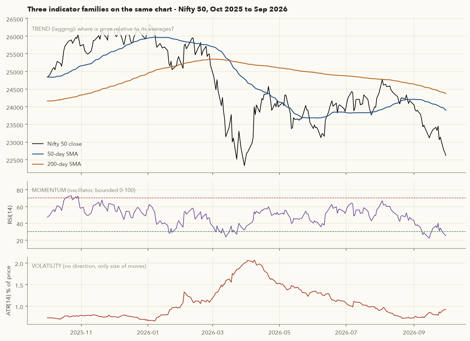
Every indicator works in one market regime and fails in another. Trend-followers make money in trends and bleed in ranges. Oscillators make money in ranges and fail badly in trends. So the first question is always "What regime is this stock in?" and only then "What is my signal?" ADX (Section 11) and the 200-day average (Section 5) exist mainly to answer the first question.
3. Moving averages: SMA and EMA
3.1 The idea in plain language
Daily closes are noisy. A moving average (MA) replaces each day's close with the average of the last n closes. Every day the oldest close drops out and the newest one comes in, so the average "moves" along the chart. The result is a smooth line that shows the underlying direction. Varsity's short summary is "the trend is your friend": the MA is a way to see that trend.
The logic: averaging cancels random day-to-day noise but keeps persistent drift. If most of the last 50 closes were higher than the 50 before them, the 50-day average is rising, and that is about as simple a definition of an uptrend as you can get. The cost of smoothing is lag. The average always trails price, and the longer the window, the bigger the lag.
3.2 Simple moving average (SMA)
- \(C\)
- A daily closing price, in ₹ (index points for Nifty). The small subscript says which day.
- \(t\)
- Today, the day you are calculating the average for. \(C_{t-1}\) is the previous session's close, \(C_{t-2}\) the one before that, and so on.
- \(n\)
- The window length: how many sessions go into the average (10, 20, 50, 200…).
- \(C_{t-n+1}\)
- The oldest close still inside the window. With \(n = 10\) it is \(C_{t-9}\): today plus the 9 sessions before it makes 10 closes. The dots \(\dots\) mean "and every close in between".
- \(SMA_t(n)\)
- The \(n\)-day simple moving average on day \(t\), in the same units as price.
How it works: add up the last \(n\) closes, including today's, and divide by \(n\). The next day, drop the oldest close, add the new one and divide again. Price above a rising SMA is the simplest sign of an uptrend. The RELIANCE example in Section 3.3 works a 10-day SMA by hand.
Every one of the n closes gets equal weight \(1/n\). One side effect is the "drop-off effect": the SMA can change direction just because a big old close falls out of the window, even if today's price did nothing unusual.
3.3 Exponential moving average (EMA)
The EMA gives more weight to recent prices. Varsity ties this to the idea that "markets discount everything", so the latest price carries the most information. It is recursive: today's EMA is yesterday's EMA nudged towards today's close by a fraction \(\alpha\), called the smoothing factor.
- \(EMA_t\)
- The exponential moving average on day \(t\) (today), in ₹.
- \(EMA_{t-1}\)
- Yesterday's EMA value. Each day's EMA is built from the previous day's.
- \(C_t\)
- Today's closing price.
- \(\alpha\)
- "Alpha", the smoothing factor: a fraction between 0 and 1. It is the weight today's close gets.
- \(n\)
- The EMA length in sessions (10, 20, …). A bigger \(n\) gives a smaller \(\alpha\) and a slower line.
- Work out \(\alpha = 2/(n+1)\).
- Seed: the first EMA value (on the \(n\)-th day) is the plain SMA of the first \(n\) closes.
- Every later day: take the gap between today's close and yesterday's EMA, \(C_t - EMA_{t-1}\), multiply it by \(\alpha\) and add the result to yesterday's EMA. That is the right-hand form of the formula. The left-hand form gives the same number: \(\alpha\) of today's close plus \((1-\alpha)\) of yesterday's EMA.
- So the EMA moves a fixed fraction of the way towards each new close. That is why it turns sooner than an SMA of the same length.
For a 10-day EMA, \(\alpha = 2/11 = 0.1818\): today's close gets 18.2% weight and the past gets the remaining 81.8%, which itself decays geometrically. For a 20-day EMA, \(\alpha = 2/21 = 0.0952\). For the first value, charting platforms usually start ("seed") the EMA with the SMA of the first n closes, and we do the same here.
Computing a 10-day SMA and EMA step by step
| Date | Close | SMA 10 | EMA 10 | What happened |
|---|---|---|---|---|
| 18 Aug 2026 | 1,322.0 | – | – | 1st close in window |
| 19 Aug | 1,311.0 | – | – | |
| 20 Aug | 1,313.2 | – | – | |
| 21 Aug | 1,316.0 | – | – | |
| 24 Aug | 1,309.8 | – | – | |
| 25 Aug | 1,317.0 | – | – | |
| 26 Aug | 1,298.0 | – | – | |
| 27 Aug | 1,282.2 | – | – | |
| 28 Aug | 1,287.0 | – | – | |
| 31 Aug | 1,277.0 | 1,303.32 | 1,303.32 | Seed: EMA = SMA of first 10 |
| 1 Sep | 1,309.0 | 1,302.02 | 1,304.35 | EMA recursion starts |
| 2 Sep | 1,313.1 | 1,302.23 | 1,305.94 | |
| 3 Sep | 1,302.5 | 1,301.16 | 1,305.32 | |
| 4 Sep | 1,322.0 | 1,301.76 | 1,308.35 | |
| … | … | … | … | |
| 30 Sep | 1,187.0 | 1,221.79 | 1,218.32 | Falling market: EMA is closer to price |
- SMA on 31 Aug: add the ten closes from 18 Aug to 31 Aug: 13,033.2. Divide by 10: \(SMA = 1{,}303.32\).
- Seed the EMA: \(EMA_{31\,Aug} = 1{,}303.32\).
- EMA on 1 Sep: \(EMA = 1{,}303.32 + 0.1818 \times (1{,}309.0 - 1{,}303.32) = 1{,}303.32 + 1.03 = 1{,}304.35\).
- SMA on 1 Sep: the 18 Aug close (1,322.0) drops out and 1,309.0 comes in: \(1{,}303.32 + (1{,}309.0 - 1{,}322.0)/10 = 1{,}302.02\). Because a high old close dropped out, the SMA fell even though price rose that day. That is the drop-off effect in action.
- By 30 Sep RELIANCE had fallen to 1,187.0. The EMA (1,218.32) had followed price down more closely than the SMA (1,221.79).
Seeding matters only at the start. An EMA computed over the full 10-year history gives 1,218.24 on 30 Sep, only 0.08 away. The influence of the starting value fades away after a few multiples of n.
3.4 SMA vs EMA on a real turn
Faster is not always earlier
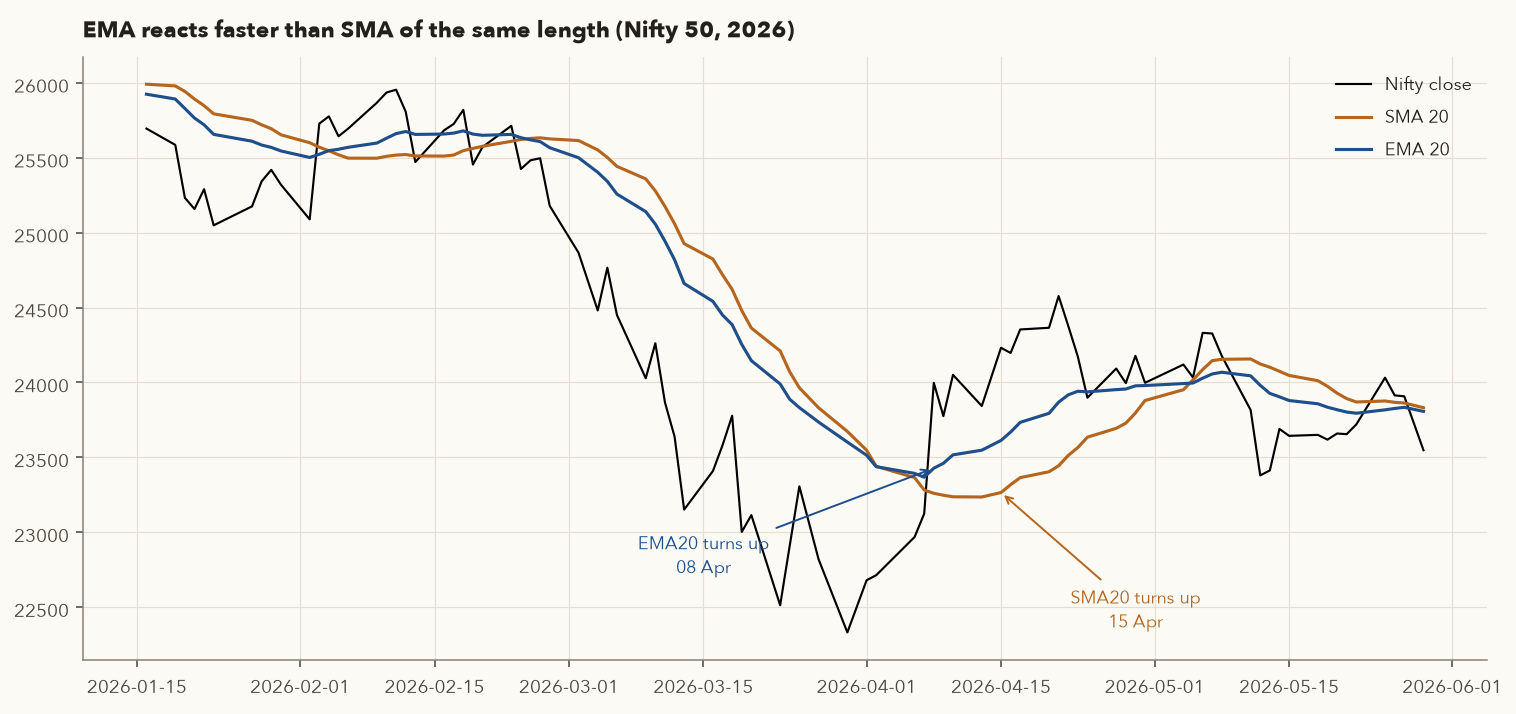
On the way up in April 2026, the EMA turned a full week before the SMA (8 Apr vs 15 Apr). On the way down the EMA was also earlier: it started falling for good on 24 Feb (Nifty 25,424.7), and the SMA only on 27 Feb (25,178.7). The days in between show the SMA's drop-off effect. On 19 Feb Nifty fell 1.4% (25,819.3 → 25,454.3), yet the 20-day SMA rose by 14.8 points, because the close leaving its window was lower still. The EMA has no window, so it fell 21.4 points that day. The cost of the EMA's speed is noise. In February alone it changed direction six times (3, 13, 16, 19, 23 and 24 Feb), against four times for the SMA. Neither one is "better". The EMA reacts sooner and makes more false turns. The SMA is steadier but can move for reasons that have nothing to do with today's price.
3.5 Choosing the length
| Length | Commonly used for | Who uses it |
|---|---|---|
| 9–21 day (often EMA) | Short-term swing direction, trailing stops on fast moves | Swing traders |
| 50 day | Intermediate trend; pullbacks to it in strong stocks are widely watched | Swing and positional traders |
| 100 day | Intermediate to long trend | Positional traders |
| 200 day | Long-term trend; the most widely quoted "bull or bear" line | Investors, fund managers, the media |
| 10 week / 30 week / 40 week | Weekly-chart equivalents of 50/150/200 days | Positional traders and investors |
- Direction: is the MA sloping up, flat or down? The slope matters more than whether price is a few rupees above or below it.
- Dynamic support/resistance: in healthy uptrends, pullbacks often stall near the 20-EMA or 50-SMA, because many traders watch those same lines.
- Stacking: price > 20-EMA > 50-SMA > 200-SMA, all rising, is a clean uptrend. Mixed order means mixed trend.
- Do not buy every close above an MA. Varsity's single-MA system (buy when price closes above the MA, sell when below) produces many small losses in sideways markets and only occasionally a big winner.
4. Moving-average crossovers and the golden/death cross
4.1 The crossover system
To reduce whipsaws, Varsity suggests using two averages instead of price vs one average. The shorter one is the "fast" MA and the longer one is the "slow" MA. Buy when the fast MA crosses above the slow MA. Exit when it crosses back below. Varsity lists these popular EMA pairs:
| Pair | Typical holding | Suits |
|---|---|---|
| 9 × 21 | Several sessions | Short swing trades |
| 25 × 50 | Several weeks | Medium-term swings |
| 50 × 100 | Several months | Intermediate trends |
| 100 × 200 | A year or more | Long-term trend following |
Varsity is clear about the profile of such systems: many small losses, a few large wins, and you must take every signal, because the edge comes from the rare big trend and you cannot know in advance which signal it will be.
4.2 Golden cross and death cross
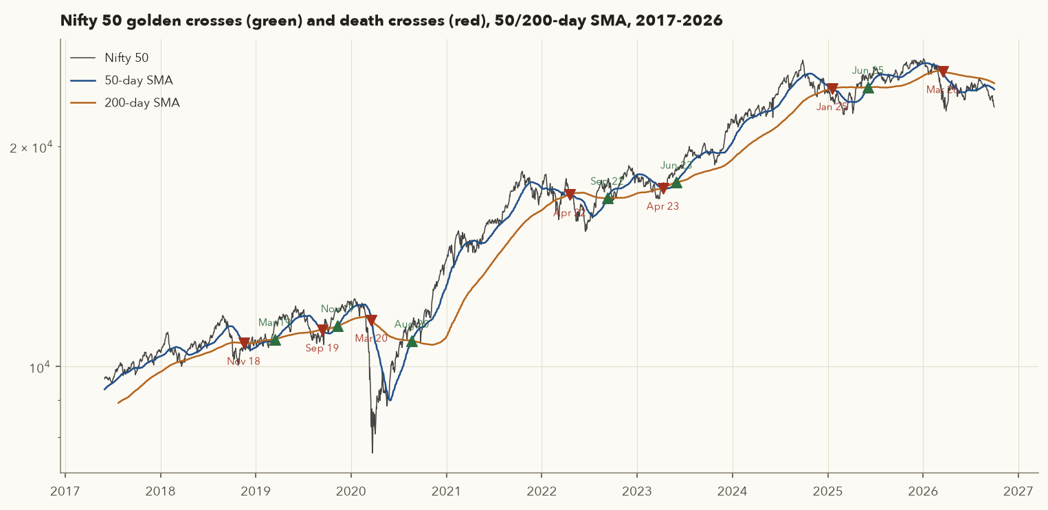
The most famous pair is the 50-day and 200-day SMA. A golden cross is the 50-day crossing above the 200-day. A death cross is the 50-day crossing below it. Financial media love these events. Here is every one of them on the Nifty 50 in our data:
| Date | Type | Nifty close | 3 months later | 6 months later | Until next cross | Change to next cross |
|---|---|---|---|---|---|---|
| 16 Nov 2018 | Death | 10,682 | −0.7% | +11.7% | 15 Mar 2019 | +7.0% |
| 15 Mar 2019 | Golden | 11,427 | +2.6% | +1.4% | 13 Sep 2019 | −3.1% |
| 13 Sep 2019 | Death | 11,076 | +10.3% | −25.4% | 11 Nov 2019 | +7.6% |
| 11 Nov 2019 | Golden | 11,913 | +1.0% | −25.9% | 19 Mar 2020 | −30.6% |
| 19 Mar 2020 | Death | 8,263 | +24.7% | +36.1% | 21 Aug 2020 | +37.6% |
| 21 Aug 2020 | Golden | 11,372 | +13.1% | +29.1% | 18 Apr 2022 | +51.0% |
| 18 Apr 2022 | Death | 17,174 | −6.5% | +1.8% | 9 Sep 2022 | +3.8% |
| 9 Sep 2022 | Golden | 17,833 | +3.7% | −3.8% | 10 Apr 2023 | −1.2% |
| 10 Apr 2023 | Death | 17,624 | +10.3% | +12.4% | 1 Jun 2023 | +4.9% |
| 1 Jun 2023 | Golden | 18,488 | +4.1% | +12.8% | 17 Jan 2025 | +25.5% |
| 17 Jan 2025 | Death | 23,203 | +4.9% | +8.0% | 4 Jun 2025 | +6.1% |
| 4 Jun 2025 | Golden | 24,620 | +0.4% | +5.7% | 17 Mar 2026 | −4.2% |
| 17 Mar 2026 | Death | 23,581 | +2.2% | −0.7% | still active on 30 Sep 2026 | −4.1% |
Did the golden cross "work" on the Nifty?
- Golden crosses: 6. Measured from each golden cross to the next death cross, only 2 of 6 were profitable (Aug 2020: +51.0%, Jun 2023: +25.5%). The average was +6.2%, and that average comes almost entirely from those two big trends. That is the "few large wins" profile Varsity describes.
- The worst one: the golden cross of 11 Nov 2019 was still "bullish" when COVID hit. By the time the death cross arrived on 19 Mar 2020, Nifty was 30.6% lower. The death cross then arrived within days of the bottom (19 Mar 2020 at 8,263; the low close was 7,610 on 23 Mar), and Nifty rose 37.6% before the next golden cross.
- Death crosses as sell signals: all 6 completed death-cross periods ended higher than where they started. The current one, active since 17 Mar 2026, is −4.1% so far. In this decade, Indian large caps recovered from falls quickly, and the 200-day average was too slow to help.
- As a full system (long when 50 > 200, otherwise cash, price index only, no costs or dividends), from 24 Jul 2017 to 30 Sep 2026: +29.3% total (CAGR 2.8%), max drawdown −41.9%, invested 74% of the time. (CAGR, the compound annual growth rate, is the steady yearly return that would produce the same total. Max drawdown is the largest fall from a previous peak in the equity curve.) Buy-and-hold over the same period: +127.0% (CAGR 9.3%), max drawdown −38.4%.
Judgement: on a broad index that kept recovering quickly, the 50/200 cross was a poor timing tool. It shines in long, grinding bear markets (2000–03 and 2008 in many markets), and this decade did not have one in India. It is still worth knowing as a regime label, and the 30 Sep 2026 state, a death cross since 17 Mar 2026, tells you the long-term trend is down.
- Treating a golden cross as a buy signal for tomorrow. It is a slow regime label. By the time it happens, much of the move is usually done.
- Using crossovers in sideways markets. The 50/200 pair crossed 13 times in 9 years on Nifty, and shorter pairs cross far more often.
- Cherry-picking signals. If you run a crossover system, take all of them, or you destroy the statistical edge that relies on catching the rare big trend.
5. Price vs the 50/200-day average as a trend filter
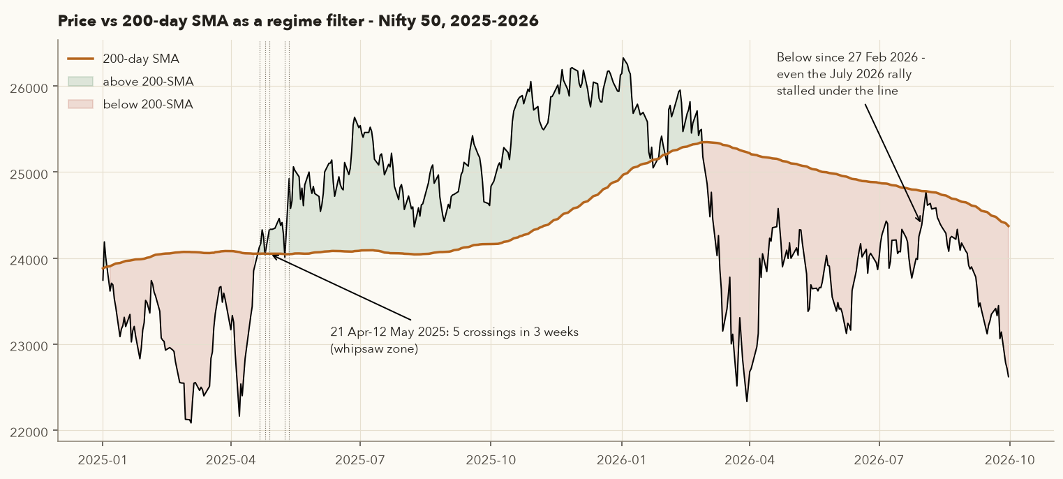
Many swing traders do not trade crossovers at all. They use "close above the 200-day SMA" (often together with "50-day above 200-day") only as a filter: long setups are considered only when it is true. The idea is that buying pullbacks inside long-term uptrends puts the larger tide behind you.
Does "above the 200-day" predict better 3-month returns?
| Nifty on day t | Days | Avg next-3-month return | % positive | Worst |
|---|---|---|---|---|
| Above 200-day SMA | 1,724 | +1.74% | 62.3% | −38.0% |
| Below 200-day SMA | 479 | +7.11% | 84.6% | −13.8% |
Nifty spent 76% of days above its 200-day average. In this sample, the days below it were followed by better returns, because almost every dip below (2018, 2020, 2022, 2023, 2025) was bought quickly. The worst three-month outcome (−38%) started when Nifty was above the line, in February 2020. Note that the "below" days come from only a handful of separate episodes, so the sample is small.
What this tells you: for an index that mean-reverts, the 200-day filter is not a return predictor. Its real jobs are (a) to keep trend-following stock strategies out of stocks in long declines (TCS in Section 6 is an example) and (b) to make you smaller and more selective when the whole market is below it, as it has been since February 2026. Test any filter on your own universe before trusting it.
- Long setups only if close > 200-SMA and 50-SMA > 200-SMA (Varsity's "trade in the direction of the trend").
- When Nifty itself is below its 200-SMA, reduce the number of open positions or the risk per trade.
- Add a "buffer" (for example 1–2% or 0.5 × ATR) before treating a cross as real, to cut whipsaws like April–May 2025.
6. RSI: Wilder's momentum oscillator
6.1 What it measures and why
Momentum is the speed of price change. If a stock rises 10% in 5 days it has high momentum. If it takes 5 months, momentum is low. J. Welles Wilder's Relative Strength Index (1978) compares the size of recent up-days with the size of recent down-days and squeezes the ratio into a 0–100 scale. When up-moves dominate, RSI is high. When down-moves dominate, it is low. (RSI has nothing to do with "relative strength vs the index", which is covered in Section 15. The name causes endless confusion.)
6.2 Calculation (14 periods, Wilder smoothing)
- \(C_t,\ C_{t-1}\)
- Today's close and the previous session's close, in ₹.
- \(G_t\)
- Today's gain: how much the close rose, or 0 if it fell. \(\max(x, 0)\) means "the larger of \(x\) and 0", so a negative change becomes 0.
- \(L_t\)
- Today's loss: how much the close fell, written as a positive number, or 0 if it rose.
- \(\overline{G},\ \overline{L}\)
- The average gain and average loss (the bar on top means "average"), in ₹ per day. \(\overline{G}_t\) is today's value, \(\overline{G}_{t-1}\) yesterday's.
- \(\textstyle\sum_{i=1}^{14} G_i\)
- The first 14 daily gains added up. \(\Sigma\) means "add up"; \(i\) counts from 1 to 14.
- \(RS\)
- Average gain divided by average loss. No units.
- \(RSI\)
- The final reading, on a 0–100 scale.
- For each day, turn the change in close into a gain or a loss. One of the two is always 0.
- Seed: once you have 14 changes (that takes 15 closes), average the 14 gains and the 14 losses separately.
- Every later day: new average = (13 × yesterday's average + today's value) ÷ 14, for gains and losses separately. This is Wilder's smoothing.
- Divide average gain by average loss to get \(RS\), then convert it: \(RSI = 100 - 100/(1+RS)\). Equal gains and losses give \(RS = 1\) and RSI 50. Mostly gains push RSI towards 100, mostly losses towards 0.
- Reading: above 70 is usually called overbought and below 30 oversold (Section 6.3).
Wilder's smoothing is just an EMA with \(\alpha = 1/14\) (not \(2/15\)). Varsity's worked example uses a plain 14-day average of gains and losses (gains 29 points, losses 10 points → avg gain 2.07, avg loss 0.714, RS 2.90, RSI 74.35). That is exactly the seed step. Charting platforms then switch to Wilder's smoothing for every later day, so their RSI has a "memory" longer than 14 days.
RSI(14) from scratch
| Date | Close | Change | Gain | Loss | Avg gain | Avg loss | RS | RSI (this window) | RSI (full history) |
|---|---|---|---|---|---|---|---|---|---|
| 11 Aug 2026 | 1,066.0 | – | – | – | – | – | – | – | 57.80 |
| 12 Aug | 1,082.0 | +16.0 | 16.0 | 0 | … 14 changes collected (12 Aug – 31 Aug) … | ||||
| 13 Aug | 1,083.0 | +1.0 | 1.0 | 0 | |||||
| 14 Aug | 1,067.7 | −15.3 | 0 | 15.3 | |||||
| 17 Aug | 1,061.2 | −6.5 | 0 | 6.5 | |||||
| 18 Aug | 1,053.0 | −8.2 | 0 | 8.2 | |||||
| 19 Aug | 1,048.6 | −4.4 | 0 | 4.4 | |||||
| 20 Aug | 1,048.0 | −0.6 | 0 | 0.6 | |||||
| 21 Aug | 1,048.7 | +0.7 | 0.7 | 0 | |||||
| 24 Aug | 1,039.5 | −9.2 | 0 | 9.2 | |||||
| 25 Aug | 1,048.0 | +8.5 | 8.5 | 0 | |||||
| 26 Aug | 1,052.0 | +4.0 | 4.0 | 0 | |||||
| 27 Aug | 1,042.9 | −9.1 | 0 | 9.1 | |||||
| 28 Aug | 1,047.5 | +4.6 | 4.6 | 0 | |||||
| 31 Aug | 1,060.0 | +12.5 | 12.5 | 0 | 3.38 | 3.81 | 0.89 | 47.02 | 54.58 |
| 1 Sep | 1,034.5 | −25.5 | 0 | 25.5 | 3.14 | 5.36 | 0.59 | 36.94 | 44.54 |
| 2 Sep | 1,020.9 | −13.6 | 0 | 13.6 | 2.91 | 5.95 | 0.49 | 32.89 | 40.28 |
| 3 Sep | 1,023.4 | +2.5 | 2.5 | 0 | 2.88 | 5.52 | 0.52 | 34.31 | 41.39 |
| … | |||||||||
| 30 Sep | 959.5 | −5.2 | 0 | 5.2 | 2.94 | 6.31 | 0.47 | 31.76 | 33.72 |
- Seed (31 Aug): the 14 gains sum to 47.3, so the average gain is 47.3/14 = 3.38. The 14 losses sum to 53.3, so the average loss is 53.3/14 = 3.81.
- \(RS = 3.38/3.81 = 0.887\), so \(RSI = 100 - 100/1.887 = 47.02\).
- 1 Sep (loss of 25.5): \(\overline G = (3.378\times13 + 0)/14 = 3.14\), \(\overline L = (3.807\times13 + 25.5)/14 = 5.36\), \(RS = 0.586\), \(RSI = 36.94\). One large down day pulled RSI down 10 points.
- Why two RSI columns? The "full history" RSI has been smoothing since 2016, so it remembers the stronger August. Our window-seeded RSI starts fresh. They differ by about 7.5 points on 31 Aug and converge to within 2 points by 30 Sep (31.76 vs 33.72). For trading, always use the full-history value. Your charting platform does the same.
6.3 Overbought and oversold
The classic reading is that RSI above 70 is overbought (a possible pullback) and below 30 is oversold (a possible bounce). Varsity's author prefers the stricter 80/20, which gives fewer but more extreme signals. Varsity also gives the opposite interpretation: if RSI stays overbought for a long time, that shows strong positive momentum, which is a reason to stay long, not to sell. The real data agrees with that more nuanced reading.
"Oversold" can keep getting more oversold
Nifty's RSI first fell below 30 on 9 Sep 2026 (close 23,431.5, RSI 26.4). Buying that "oversold" reading would have been early. On 30 Sep Nifty closed at 22,620.4 (−3.5%) with RSI 25.3, and it spent 9 sessions of September below 30. In a downtrend (Nifty had been below its 200-day SMA since February), oversold readings describe the trend. They do not predict a turn.
6.4 RSI ranges shift with the trend
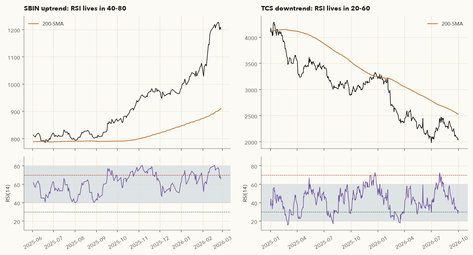
A very useful practical idea, popularised by Andrew Cardwell and Constance Brown, is that in a strong uptrend RSI tends to oscillate between about 40 and 80 and rarely reaches 30. In a downtrend it oscillates between about 20 and 60 and rarely reaches 70. So in an uptrend, a dip to 40–45 is the "oversold" buy zone, and in a downtrend a rally to 55–60 is the "overbought" zone.
6.5 Divergence
A bullish divergence happens when price makes a lower low but RSI makes a higher low. The selling pushed price lower, but with less force than the previous wave. A bearish divergence is a higher high in price with a lower high in RSI. Divergence is a warning that momentum is fading. It is not an entry signal by itself, because divergences can repeat two or three times before price actually turns.
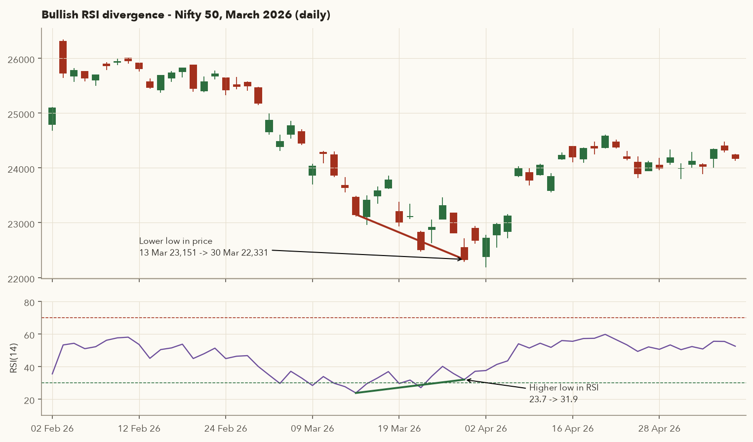
Bullish RSI divergence at the March 2026 low
- First low: 13 Mar 2026, close 23,151.1, RSI 23.7 (deeply oversold; RSI had first dropped below 30 on 4 Mar).
- Second, lower low: 30 Mar 2026, close 22,331.4 (820 points lower), but RSI only 31.9, a higher low.
- Confirmation: at the second low RSI was already back above 30 (31.9), unlike the 23.7 reading two weeks earlier. On 1 Apr Nifty closed higher at 22,679.4 (RSI 37.0); the 2 Apr intraday dip to 22,182.6 closed well off the low (22,713.1) and turned out to be the final bottom. On 8 Apr Nifty gapped up and closed 3.8% higher, which was the price confirmation.
- Outcome: from the 30 Mar close to the 21 Apr close (24,576.6) Nifty rose +10.1%.
- Caution: on 23 Mar (close 22,512.7, RSI 26.9) a trader could already have seen a "divergence" against 13 Mar. Price still fell another 0.8% to 30 Mar. Divergence tells you the falls are getting weaker. Price structure (a higher low, a break of a down-trendline) tells you when.
- Selling a strong stock just because RSI > 70: ADANIENT's RSI first crossed 70 on 23 Apr 2026 at 2,300. It closed at 3,048.2 on 5 Jun (Section 8.4).
- Buying a falling stock because RSI < 30: TCS spent 17.8% of 2025–26 below 30 while it halved.
- Changing the lookback until the past looks perfect. Shorter lookbacks (5, 7) make RSI jumpy. Longer ones (20+) make it sluggish. Pick one setting and test it.
7. MACD: trend and momentum in one
7.1 Construction
Gerald Appel's Moving Average Convergence Divergence measures the gap between a fast and a slow EMA. When the 12-day EMA pulls away above the 26-day EMA, upward momentum is building (the averages diverge). When they come back together, momentum is fading (they converge).
- \(EMA_{12}(C)_t\)
- The 12-day EMA of closing prices on day \(t\) (Section 3.3): the "fast" average.
- \(EMA_{26}(C)_t\)
- The 26-day EMA of closes: the "slow" average.
- \(MACD_t\)
- The MACD line: fast EMA minus slow EMA, in ₹ (points for Nifty). Positive when the fast average is above the slow one.
- \(Signal_t\)
- The signal line: a 9-day EMA of the MACD line itself, i.e. a smoothed, slower copy of MACD.
- \(Histogram_t\)
- MACD minus signal, drawn as bars around zero.
- Each day, compute the 12-day and 26-day EMAs of the close and subtract the slow one from the fast one. That is the MACD line.
- Treat the MACD values as a new series and take its 9-day EMA. That is the signal line.
- Subtract the signal line from MACD to get the histogram. It is positive when MACD is above its signal line (momentum improving) and negative when below. The usual setting is written (12, 26, 9). The ADANIENT table below shows real values.
MACD is in price units (rupees for a stock, points for Nifty), so a value of 100 on a ₹3,000 stock is not comparable with 100 on a ₹300 stock. Compare MACD only with its own history, or divide by price.
7.2 Signals
- Signal-line crossover (Varsity's main signal): MACD crosses above the signal line → bullish. Crosses below → bearish. Equivalent to the histogram changing sign.
- Zero-line (centreline) crossover: MACD crosses above 0 → the 12-EMA is now above the 26-EMA, so the medium-term trend has turned up. Slower but more reliable.
- Histogram: shrinking bars mean momentum is fading before the crossover happens. That makes the histogram the "earliest" part of MACD.
- Divergence: same idea as RSI. Price makes a lower low while the MACD line or histogram makes a higher low.
MACD table around a major turn
| Date | Close | EMA 12 | EMA 26 | MACD | Signal | Histogram |
|---|---|---|---|---|---|---|
| 30 Mar 2026 | 1,758.8 | 1,896.69 | 1,981.02 | −84.33 | −66.55 | −17.77 |
| 1 Apr | 1,842.5 | 1,888.36 | 1,970.76 | −82.40 | −69.72 | −12.68 |
| 2 Apr | 1,834.2 | 1,880.02 | 1,960.64 | −80.62 | −71.90 | −8.72 |
| 6 Apr | 1,902.2 | 1,883.44 | 1,956.31 | −72.88 | −72.10 | −0.78 |
| 7 Apr | 1,882.1 | 1,883.23 | 1,950.82 | −67.59 | −71.19 | +3.61 |
| 8 Apr | 2,043.8 | 1,907.93 | 1,957.70 | −49.77 | −66.91 | +17.14 |
| 13 Apr | 2,129.0 | 1,979.83 | 1,984.50 | −4.67 | −42.98 | +38.30 |
| 15 Apr | 2,144.4 | 2,005.15 | 1,996.35 | +8.80 | −32.62 | +41.42 |
- Histogram shrinking: from −17.77 on 30 Mar to −0.78 on 6 Apr. Downward momentum was fading while price was still near its low.
- Signal-line crossover (7 Apr): \(MACD = 1{,}883.23 - 1{,}950.82 = -67.59\), which is now above the signal line (−71.19), so the histogram turns positive at +3.61. Bullish cross at a close of 1,882.1.
- Zero-line crossover (15 Apr): the 12-EMA (2,005.15) moved above the 26-EMA (1,996.35) at 2,144.4, about 14% above the signal-line entry.
- Exit: the next bearish signal-line cross came on 8 Jun 2026 at 2,970.0. From 1,882.1 that is +57.8%.
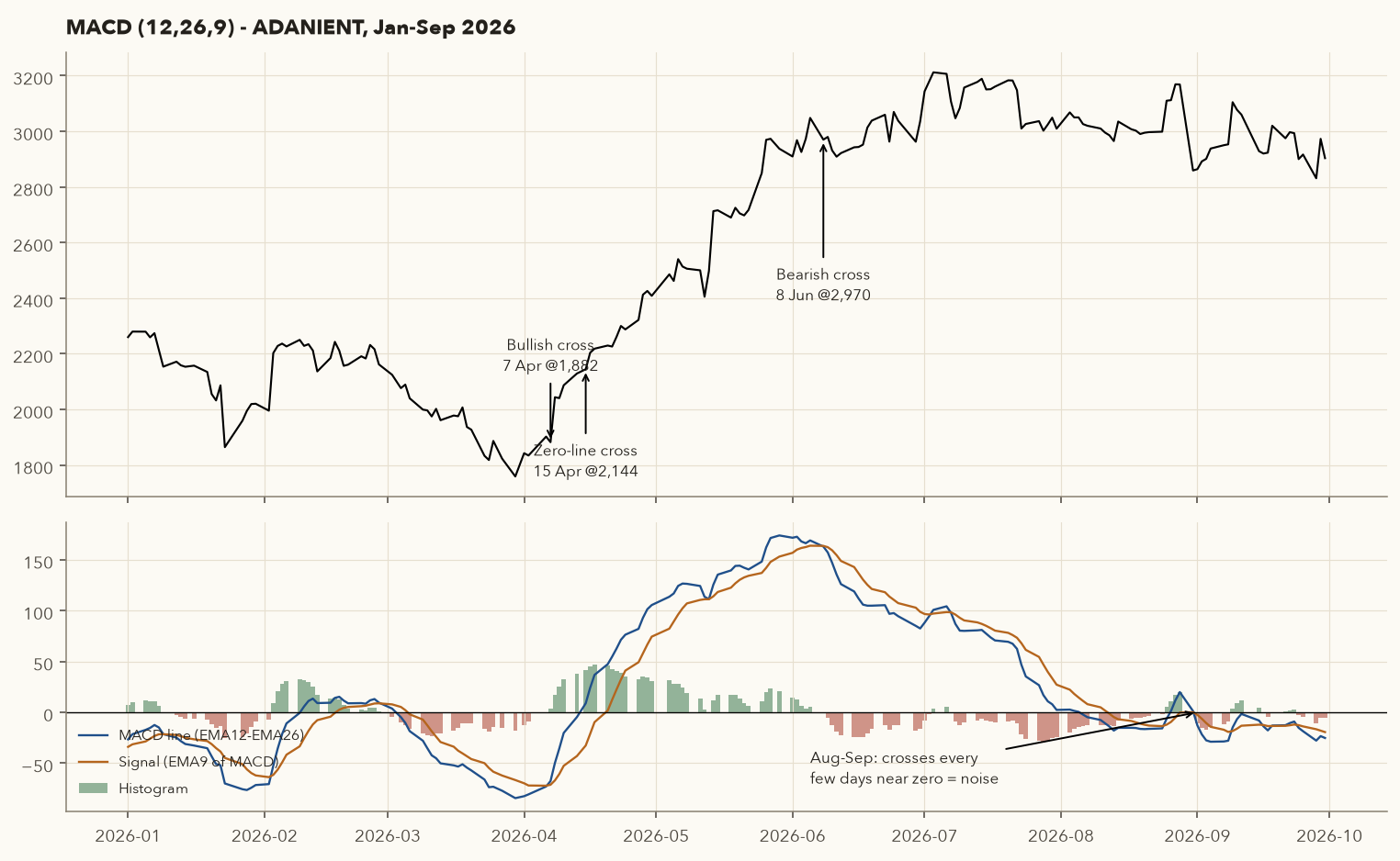
All long-only MACD signal-line trades in 2026
| Entry | Entry price | Exit | Exit price | Result |
|---|---|---|---|---|
| 3 Feb | 2,202.6 | 2 Mar | 2,124.6 | −3.5% |
| 7 Apr | 1,882.1 | 8 Jun | 2,970.0 | +57.8% |
| 3 Jul | 3,212.1 | 7 Jul | 3,107.2 | −3.3% |
| 25 Aug | 3,110.0 | 1 Sep | 2,863.9 | −7.9% |
| 9 Sep | 3,104.7 | 16 Sep | 2,920.0 | −5.9% |
| 18 Sep | 3,020.0 | 24 Sep | 2,900.0 | −4.0% |
One big winner and five losers. Once the trend stalled (July–September), MACD crossed back and forth near zero every few days. This is the classic trend-follower profile, and it is why Varsity warns that MACD "works in trending markets but performs poorly in sideways markets". A practical improvement is to accept signal-line crosses only in the direction of the zero line (longs only when MACD > 0) or only when ADX > 20–25.
MACD histogram divergence
Nifty closes on 13 Mar, 23 Mar and 30 Mar 2026 were 23,151 → 22,513 → 22,331 (lower lows). The MACD histogram on those dates was −193.0 → −129.1 → −65.0 (higher lows). The bars were shrinking even as price fell. The same signal as the RSI divergence in Section 6.5 appeared, from a different formula. That is unsurprising, since both measure momentum (Section 18).
8. Bollinger Bands: volatility envelopes
8.1 Construction
John Bollinger's bands place an envelope around a 20-day SMA at ±2 standard deviations of the last 20 closes. Standard deviation (SD) measures how spread out the closes are. When the stock is calm the bands squeeze together, and when it is volatile they widen.
- \(C\)
- Today's close, in ₹. \(C_{t-i}\) is the close \(i\) sessions ago.
- \(Mid_t\)
- The middle band: the 20-day SMA of closes on day \(t\).
- \(\sigma_t\)
- "Sigma", the standard deviation of the last 20 closes, in ₹: how far closes typically sit from their average. \(\textstyle\sum_{i=0}^{19}\) adds up the 20 terms from \(i = 0\) (today) to \(i = 19\) (19 sessions ago).
- \(Upper,\ Lower\)
- The upper and lower bands, 2 standard deviations above and below the middle line.
- \(\%B\)
- Where today's close sits between the bands, as a fraction.
- \(Bandwidth\)
- The gap between the bands as a fraction of the middle line, usually shown as a %.
- Average the last 20 closes. That is \(Mid\).
- For each of those 20 closes, subtract \(Mid\) and square the result (squaring makes every gap positive). Average the 20 squares and take the square root. That is \(\sigma\). Dividing by 20 gives the "population" standard deviation, which the framework uses.
- Upper band = \(Mid + 2\sigma\), lower band = \(Mid - 2\sigma\).
- \(\%B\) = distance of the close above the lower band ÷ full band width. Bandwidth = band width ÷ \(Mid\). The next paragraph explains how to read both, and the HAL example below computes all of them.
%B tells you where price sits inside the bands: 0 = on the lower band, 0.5 = on the middle line, 1 = on the upper band, above 1 = outside the upper band. Bandwidth measures how wide the bands are relative to price, and a multi-month low in bandwidth is a "squeeze".
The logic: if closes were normally distributed, about 95% would fall within ±2 SD. Price is not normally distributed (it trends and has fat tails), so the bands are best read as "what is unusual relative to the last month", not as a probability statement.
Computing the bands, %B and bandwidth
- Last 20 closes (24 Jun – 21 Jul 2026): 4,500.2, 4,368.9, 4,368.7, 4,342.8, 4,381.2, 4,434.4, 4,434.0, 4,428.9, 4,440.6, 4,400.3, 4,364.7, 4,378.9, 4,506.8, 4,511.3, 4,442.4, 4,420.5, 4,433.8, 4,500.7, 4,491.0, 4,581.7.
- Mean: \(Mid = 4{,}436.59\). Population SD: \(\sigma = 60.80\).
- \(Upper = 4{,}436.59 + 2 \times 60.80 = 4{,}558.2\); \(Lower = 4{,}436.59 - 121.6 = 4{,}314.98\).
- \(\%B = (4{,}581.7 - 4{,}314.98)/(4{,}558.2 - 4{,}314.98) = 266.7/243.2 = 1.097\). The close was above the upper band.
- \(Bandwidth = 243.2 / 4{,}436.59 = 5.48\%\). Five days earlier (16 Jul) it was 4.55%, the lowest in 126 sessions (about 6 months). Compare 9.75% on 1 Jul.
8.2 Varsity's way: mean reversion in ranges
Varsity teaches Bollinger Bands as a mean-reversion tool. Price at the upper band is "expensive" relative to its average, so short it with a target at the middle line. Price at the lower band is "cheap", so buy it with a target at the middle line. Varsity also warns that this fails when the bands expand during a strong trend ("envelope expansion"). Bollinger's own guidance adds two more patterns, the squeeze and the band walk.
In the NSE cash segment you can sell shares you do not own only intraday. A short sale must be bought back the same day, or the undelivered shares go to the exchange auction at a penalty price. So any "short" in this chapter (Bollinger upper-band fades, ADX/MACD sell signals) held for days needs stock futures or options (Chapters 9–10). As a beginner swing trader in cash, use the long side of these rules, and read sell signals as "exit or do not buy".
8.3 The squeeze, and the head-fake
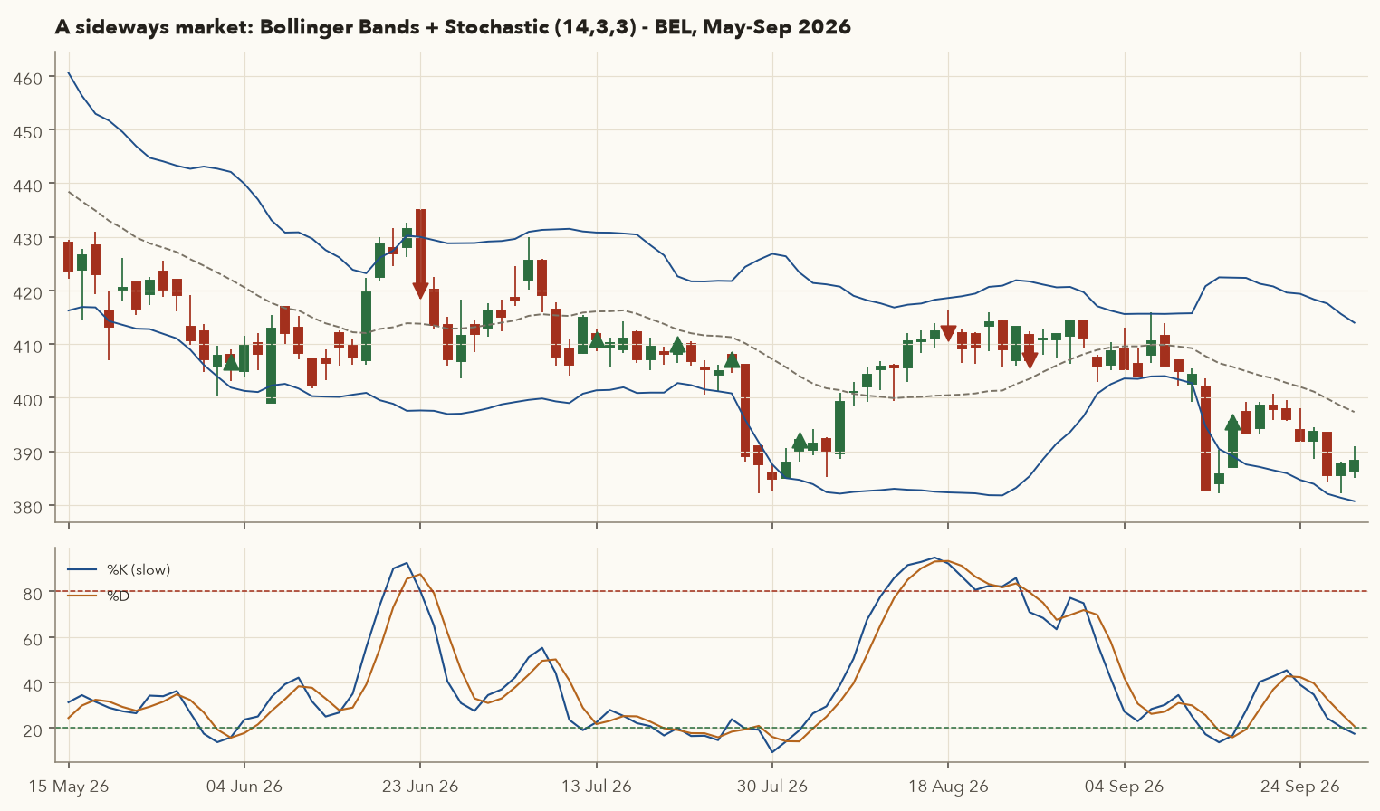
Volatility tends to alternate: quiet periods are followed by active ones. A squeeze (bandwidth at a multi-month low) says a big move is getting more likely. It does not say in which direction. Traders wait for a close outside a band and then follow it. Bollinger himself warned about the head-fake: a first break one way that reverses into the real move the other way.
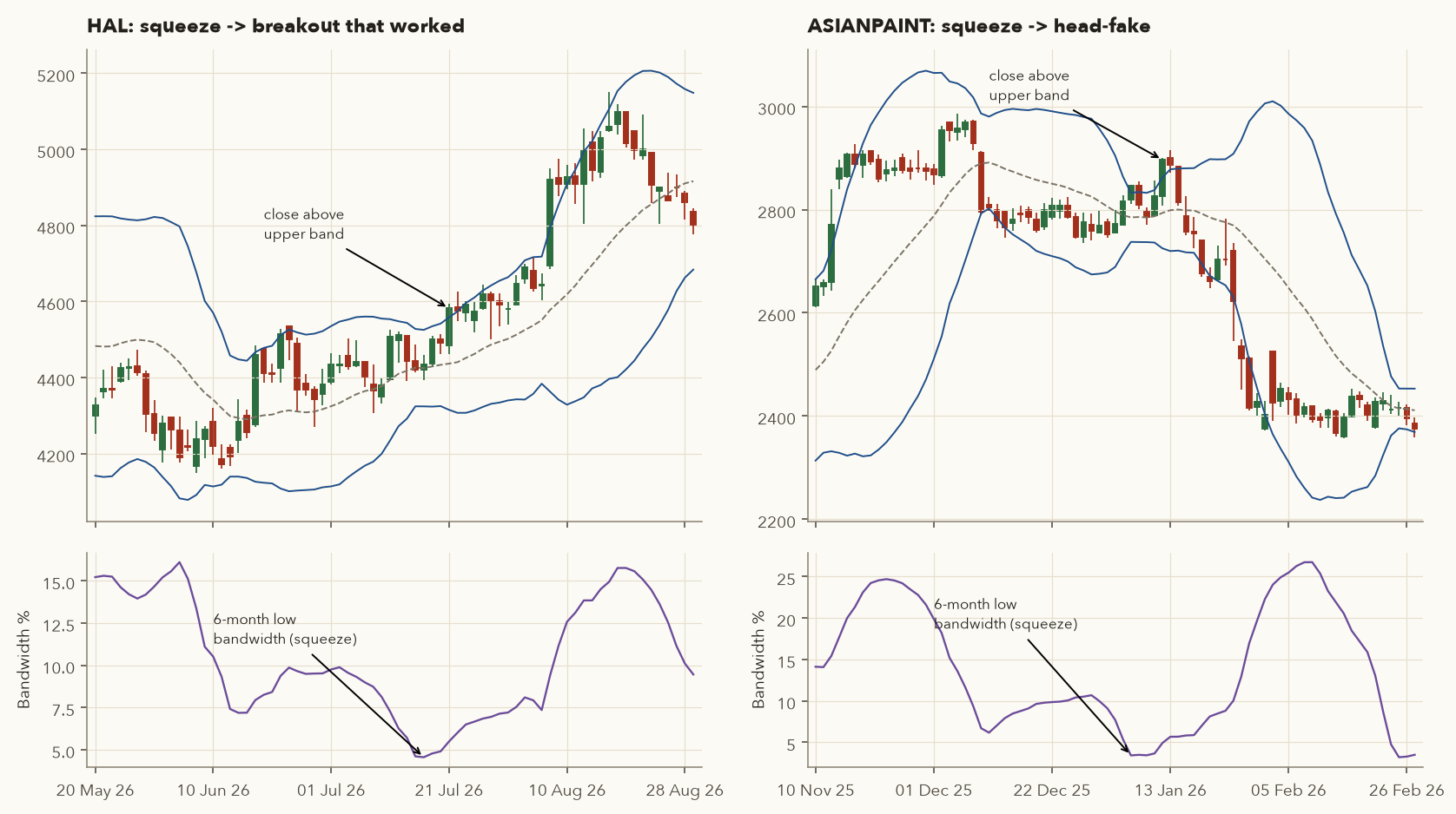
How often does a squeeze breakout follow through?
We scanned 35 stocks (TRENT and TMPV excluded because of corporate-action data artefacts) for every 126-day bandwidth low, then took the first close outside a band within 10 sessions and measured the move over the next 20 sessions in the breakout direction.
A squeeze on its own was roughly a coin flip in this sample (39 upside breaks, 20 followed through; 47 downside breaks, 26 followed through). The squeeze is a "pay attention" flag. The edge has to come from elsewhere: the bigger trend, volume on the breakout (HAL's real move came with 7.8× average volume on 6 Aug, see Section 13), and a tight stop if the break fails.
8.4 The band walk
In a strong trend price can "walk" along the upper band, closing near or above it day after day. Shorting the upper-band touch in that situation is exactly Varsity's "envelope expansion" failure.
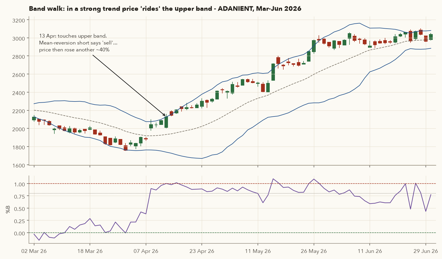
"Touches the upper band, so sell" in a trend
- On 13 Apr 2026 ADANIENT closed at 2,129.0 with %B = 1.001, exactly on the upper band. A mean-reversion trader would short it, targeting the middle band.
- From 8 Apr to 5 Jun, %B was at or above 0.8 on 36 of 40 sessions, with 6 closes above the upper band.
- Price went from 2,043.8 (8 Apr) to 3,048.2 (5 Jun). The short from 2,129 would have lost about 43%.
- What should have warned you: the bands were widening (bandwidth rising), price was above a rising 20-SMA, and the MACD and Supertrend had both turned up (Sections 7 and 12). Fade the bands only when ADX is low and the bands are flat.
9. Stochastic oscillator (brief)
George Lane's Stochastic asks: where is today's close within the high–low range of the last 14 days? In an uptrend, closes tend to be near the top of the recent range, and in a downtrend near the bottom.
- \(C_t\)
- Today's close, in ₹.
- \(LL_{14}\)
- The lowest low of the last 14 sessions, today included.
- \(HH_{14}\)
- The highest high of the last 14 sessions, today included.
- \(\text{raw }\%K\)
- Where today's close sits inside that 14-day range: 0 = at the lowest low, 100 = at the highest high.
- \(SMA_3(\dots)\)
- A plain 3-day average of whatever is in the brackets.
- \(\%K_{slow}\)
- The 3-day average of raw %K. This is the "%K" line on most charts.
- \(\%D\)
- The 3-day average of slow %K: a slower signal line.
- Find the 14-day range: highest high minus lowest low.
- Take how far today's close is above the lowest low, divide by the range and multiply by 100. That is raw %K.
- Average the last three raw %K values to get slow %K. Average the last three slow %K values to get %D. These two averaging steps are the "3, 3" in the (14, 3, 3) setting.
- Plot slow %K and %D together, both on a 0–100 scale. The next paragraph gives the overbought and oversold levels and the crossover signals.
Above 80 is overbought and below 20 is oversold. A buy signal is %K crossing above %D while below 20, and a sell signal is %K crossing below %D while above 80.
Stochastic step by step
| Date | High | Low | Close | 14-day LL | 14-day HH | raw %K | %K (slow) | %D |
|---|---|---|---|---|---|---|---|---|
| 15 Sep 2026 | 403.65 | 382.90 | 382.90 | 382.90 | 416.00 | 0.00 | 17.29 | 25.66 |
| 16 Sep | 390.20 | 382.10 | 385.75 | 382.10 | 416.00 | 10.77 | 13.74 | 18.74 |
| 17 Sep | 395.90 | 387.00 | 395.45 | 382.10 | 416.00 | 39.38 | 16.72 | 15.92 |
| 18 Sep | 399.20 | 393.30 | 393.30 | 382.10 | 416.00 | 33.04 | 27.73 | 19.39 |
- 17 Sep raw %K: \(100 \times (395.45 - 382.10)/(416.00 - 382.10) = 100 \times 13.35/33.90 = 39.38\).
- Slow %K: average of the last three raw values \((0.00 + 10.77 + 39.38)/3 = 16.72\).
- %D: average of the last three slow %K values \((17.29 + 13.74 + 16.72)/3 = 15.92\).
- %K (16.72) crossed above %D (15.92) below 20, which is a buy signal at 395.45. By 30 Sep, nine sessions later and the end of our data, BEL was 1.8% lower. In this range, the 6 buy signals (May–Sep 2026) were higher 10 sessions later only twice (the last one measured to 30 Sep). The 3 sell signals were each followed by small declines (−3.0%, −0.2%, −0.2%).
Use it for: timing entries inside a known range or a pullback within a trend. Do not use it with RSI and %B together. Section 18 shows the three are 0.83–0.89 correlated, so they mostly repeat each other.
10. ATR: measuring volatility for stops and position size
10.1 True range
Wilder's Average True Range measures how much a stock typically moves in a day, including gaps. The plain high-minus-low range ignores overnight gaps, which is a serious omission in India, where results, global news and overnight moves in GIFT Nifty (formerly SGX Nifty) cause frequent gap opens. True range uses the largest of three distances:
- \(H_t,\ L_t\)
- Today's high and low, in ₹.
- \(C_{t-1}\)
- The previous session's close.
- \(|x|\)
- The absolute value: the size of \(x\) ignoring its sign, so \(|-285.2| = 285.2\).
- \(TR_t\)
- Today's true range, in ₹: the largest (\(\max\)) of the three distances in the brackets.
- \(ATR_t\)
- The 14-day average true range on day \(t\), in ₹. \(ATR_{t-1}\) is yesterday's value.
- Work out three distances: high minus low, high to the previous close, and low to the previous close (the last two ignoring sign). The true range is the biggest. On a normal day it is just high minus low. After a gap, one of the other two is larger.
- Seed: the first ATR is the plain average of the first 14 true ranges.
- Every later day: ATR = (13 × yesterday's ATR + today's TR) ÷ 14. This is the same Wilder smoothing as in RSI.
- Read ATR as "a typical day's move in rupees". Divide it by price to compare stocks (Section 10.3).
Why true range matters: the 8 April gap-up
| Date | High | Low | Prev close | H − L | |H − prev C| | |L − prev C| | TR | ATR 14 |
|---|---|---|---|---|---|---|---|---|
| 6 Apr 2026 | 22,998.3 | 22,542.9 | 22,713.1 | 455.4 | 285.2 | 170.2 | 455.4 | 467.5 |
| 7 Apr | 23,153.8 | 22,719.3 | 22,968.2 | 434.5 | 185.6 | 248.9 | 434.5 | 465.1 |
| 8 Apr | 24,025.2 | 23,828.5 | 23,123.7 | 196.7 | 901.5 | 704.8 | 901.5 | 496.3 |
| 9 Apr | 23,990.8 | 23,682.8 | 23,997.3 | 307.9 | 6.6 | 314.5 | 314.5 | 483.3 |
| 10 Apr | 24,074.1 | 23,856.3 | 23,775.1 | 217.7 | 299.0 | 81.2 | 299.0 | 470.2 |
- On 8 Apr Nifty gapped up. The day's own range was only 196.7 points, but the move from the previous close to the high was 901.5. The true range is 901.5, not 196.7.
- \(ATR_{8\,Apr} = (465.1 \times 13 + 901.5)/14 = (6{,}046.3 + 901.5)/14 = 496.3\).
- ATR as a % of price: \(496.3/23{,}997.3 = 2.07\%\), the highest of the past year (Figure 4.1).
10.2 Using ATR for stops
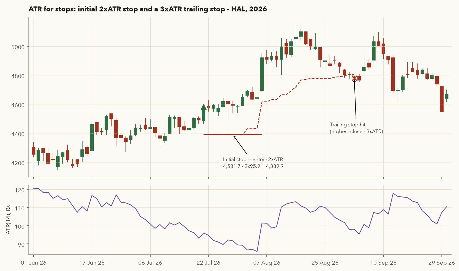
A stop placed inside a stock's normal daily noise gets hit by randomness, not by being wrong. ATR tells you how wide that noise is. Varsity's rule: place the stop at least one ATR from entry (long: entry − ATR; short: entry + ATR). Swing traders commonly use 1.5–3 × ATR, and a chandelier stop trails the stop at "highest close since entry − 3 × ATR". (Chuck LeBeau's original uses the highest high and a 22-day ATR. Using closes, as we do here, is a common variant that is slightly less likely to be stopped by one intraday spike.)
ATR stop and position size on the squeeze breakout
- Entry: close of 21 Jul 2026 = ₹4,581.70. ATR(14) that day = ₹95.92.
- Initial stop (2 × ATR): \(4{,}581.70 - 2 \times 95.92 = \text{₹}4{,}389.87\). Risk per share = ₹191.83.
- Position size for a ₹5,00,000 account risking 1% (₹5,000) per trade: \[ Qty = \left\lfloor \frac{5{,}000}{191.83} \right\rfloor = 26 \text{ shares} \] Position value \(26 \times 4{,}581.70 = \text{₹}1{,}19{,}124\), or 23.8% of capital. Actual risk \(26 \times 191.83 = \text{₹}4{,}988\).
- Trailing (chandelier): stop = highest close since entry − 3 × ATR, never lowered. The highest close was 5,099.0 (18 Aug). The stop ratcheted up to ₹4,805.48 and was broken on 2 Sep at 4,780.0.
- Result: traders measure outcomes in R, multiples of the initial risk per share (here ₹191.83). \((4{,}780.0 - 4{,}581.7)/191.83 = +1.03R\), about ₹5,156 on 26 shares before costs. The trailing stop gave back part of the peak gain, which is the price of staying in for a bigger trend.
ATR tells you if one futures lot fits your risk budget
- HAL's futures lot size in the NSE F&O bhavcopy of 30 Sep 2026 is 150 shares. (Lot sizes are revised periodically. Check the current NSE contract specification before you trade.)
- Using the same 2 × ATR stop (₹191.83 per share), the risk per lot is \(150 \times 191.83 = \text{₹}28{,}775\).
- For a ₹5,00,000 account that is 5.75% risk on a single trade, nearly six times the 1% rule. To keep one lot within 1%, you would need about \(28{,}775 / 0.01 = \text{₹}28.8\) lakh of capital.
- The contract's notional value (the full market value of the shares the lot represents) is \(150 \times 4{,}581.70 = \text{₹}6.87\) lakh, larger than the whole account. That is leverage, and it is why Chapter 9 treats futures sizing separately.
Lesson: with futures you cannot buy "26 shares". You trade whole lots. If ATR × multiple × lot size exceeds your risk budget, the correct position size is zero.
10.3 ATR as a comparison tool
Raw ATR depends on the price level, so convert it to a percentage of price to compare stocks. On 30 Sep 2026, HAL's ATR was ₹110.36 (2.36% of its ₹4,668 price) and HDFCBANK's was ₹13.96 (1.97% of ₹708.70). A fixed "5% stop" is therefore about 2.1 ATRs for HAL but 2.5 ATRs for HDFCBANK. ATR-based stops adjust automatically for each stock's personality.
11. ADX and the DMI: is there a trend at all?
11.1 The idea
Wilder's Directional Movement system has three lines. +DI measures upward pressure (how much today's high exceeds yesterday's). −DI measures downward pressure (how much today's low undercuts yesterday's). ADX is a smoothed measure of how far apart +DI and −DI are. ADX tells you the strength of a trend, not its direction. A falling market with strong selling has a high ADX too.
- \(H_t,\ L_t\)
- Today's high and low, in ₹. \(H_{t-1},\ L_{t-1}\) are the previous session's.
- \(up\)
- How far today's high is above yesterday's high (negative if it is below).
- \(down\)
- How far today's low is below yesterday's low (negative if it is above).
- \({+DM},\ {-DM}\)
- Plus and minus directional movement for the day, in ₹. Only the bigger of \(up\) and \(down\) counts, and only if it is positive. The other is 0. On an inside day (lower high, higher low) both are 0.
- \(\text{Wilder}_{14}(\dots)\)
- Wilder's 14-day smoothing, as in RSI and ATR: start with a plain 14-day average, then new = (13 × old + today) ÷ 14.
- \(ATR_{14}\)
- The 14-day average true range (Section 10).
- \({+DI},\ {-DI}\)
- Plus and minus directional indicators: smoothed +DM and −DM as a percentage of ATR.
- \(DX\)
- Directional index: the gap between +DI and −DI as a percentage of their sum. Near 0 = the two sides are balanced, near 100 = one side dominates.
- \(ADX\)
- Average directional index: DX smoothed over 14 days, on a 0–100 scale.
- Each day, compare today's bar with yesterday's to get \(up\) and \(down\). The larger one, if positive, becomes +DM or −DM. The other is 0.
- Smooth +DM, −DM and the true range with Wilder's 14-day method. Then +DI = 100 × smoothed +DM ÷ ATR, and the same for −DI.
- DX = 100 × the gap between +DI and −DI (ignoring sign) ÷ their sum. Smooth DX the same way to get ADX.
- Reading: ADX above 25 means a strong trend, below 20 means little or no trend. ADX does not give direction. Which DI is on top tells you that (table below).
| ADX (Varsity's bands) | Meaning | Which tools to favour |
|---|---|---|
| Below 20 | Weak or no trend | Range tools: Bollinger fades, Stochastic, support/resistance |
| 20–25 | Grey zone | Wait or trade small |
| Above 25 | Strong trend (direction from +DI vs −DI) | Trend tools: MAs, Supertrend, breakouts, pullback entries |
Varsity's trade rule: buy when ADX is above 25 and +DI is above −DI. Sell or short when ADX is above 25 and −DI is above +DI. Stop at the low (or high) of the signal candle.
Computing ADX on the day it crossed 25
| Date | High | Low | Close | +DM | −DM | TR | ATR | +DI | −DI | DX | ADX |
|---|---|---|---|---|---|---|---|---|---|---|---|
| 18 Aug 2025 | 14,125 | 13,664 | 14,068 | 1,169 | 0 | 1,189 | 285.59 | 45.77 | 11.32 | 60.34 | 12.52 |
| 19 Aug | 14,270 | 13,979 | 14,250 | 145 | 0 | 291 | 285.97 | 46.06 | 10.50 | 62.88 | 16.12 |
| 20 Aug | 14,362 | 14,200 | 14,221 | 92 | 0 | 162 | 277.12 | 46.51 | 10.06 | 64.44 | 19.57 |
| 21 Aug | 14,401 | 14,156 | 14,280 | 0 | 44 | 245 | 274.82 | 43.55 | 10.56 | 60.96 | 22.53 |
| 22 Aug | 14,370 | 14,230 | 14,349 | 0 | 0 | 140 | 265.19 | 41.90 | 10.16 | 60.96 | 25.27 |
- 18 Aug: high rose by 1,169 versus the prior day, and the low did not fall, so +DM = 1,169 and −DM = 0. This was a big gap-up day (a TR of 1,189), when autos rallied on GST-cut expectations.
- 22 Aug: \(DX = 100 \times |41.90 - 10.16|/(41.90 + 10.16) = 100 \times 31.74/52.06 = 60.96\).
- \(ADX = (22.53 \times 13 + 60.96)/14 = 25.27\). It crossed 25 with +DI above −DI, which is Varsity's buy condition, at a close of 14,349.
- Note the lag: +DI had already moved above −DI on 12 Aug at 12,840, when ADX was only 7.4. ADX confirms a trend that is already under way.
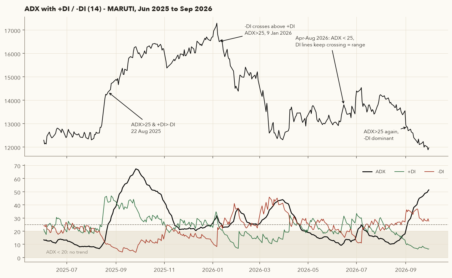
Reading the four regimes
- Uptrend: buy signal 22 Aug 2025 at 14,349. ADX peaked near 67 in late September. The closing high was 16,703 on 24 Dec 2025 (+16.4% from the signal).
- Downtrend: on 9 Jan 2026 −DI (22.8) crossed above +DI (22.7) with ADX 26.6 at 16,501, a sell signal. MARUTI fell to 12,306 by 30 Mar 2026 (−25.4%).
- Range: from 20 Apr to 2 Sep 2026, ADX averaged 15.5 and never exceeded 25.0, while the DI lines crossed 13 times. Every DI crossover in that period was noise. ADX correctly said "no trend, step aside".
- New downtrend: ADX rose above 25 again on 3 Sep 2026 (25.2) with −DI at 34.7 vs +DI at 10.4, close 12,857. By 30 Sep: close 11,967, ADX 51.4.
12. Supertrend
Supertrend (by Olivier Seban) is an ATR-based trailing line. In an uptrend it sits below price as a green line and only moves up. When price closes below it, the line flips above price, turns red, and from then on only moves down. It is a trend-following system and a trailing stop in one.
- \(H_t,\ L_t\)
- Today's high and low, in ₹. \(\frac{H_t + L_t}{2}\) is the midpoint of today's bar.
- \(ATR_n\)
- The \(n\)-day average true range on day \(t\) (Section 10), in ₹.
- \(n\)
- The ATR period in sessions: 10 in our examples, 7 on Kite's default.
- \(m\)
- The multiplier: how many ATRs the bands sit from the midpoint (3 in our examples).
- \(\text{BasicUpper}_t,\ \text{BasicLower}_t\)
- Today's raw bands: the midpoint plus or minus \(m\) ATRs.
- \(\text{FinalLower}_t\)
- The ratcheted lower band, the line used in long mode. \(\text{FinalLower}_{t-1}\) is yesterday's value.
- \(\text{FinalUpper}_t\)
- The ratcheted upper band, the line used in short mode.
- \(C_{t-1}\)
- The previous session's close.
- Each day, compute the basic bands: midpoint of the bar ± \(m\) × ATR.
- Ratchet the lower band: take today's basic lower band only if it is higher than yesterday's final lower band. Otherwise keep yesterday's value, so the line can only rise. The exception: if yesterday's close was already below the old line, the band resets to today's basic value.
- FinalUpper mirrors this: it can only fall, unless the previous close was above it.
- In long mode, Supertrend = FinalLower (the green line under price). A close below it flips to short mode, where Supertrend = FinalUpper (the red line above price). A close above FinalUpper flips it back to long.
Settings: Kite's default, which Varsity uses, is period 7, multiplier 3, and Varsity suggests keeping the multiplier between 3 and 4. TradingView's built-in default is period 10, multiplier 3. A larger multiplier means fewer flips and later exits. The examples here use (10, 3), so your Kite chart with (7, 3) will flip on slightly different days.
The flip from short to long
| Date | Close | (H+L)/2 | ATR 10 | Basic upper | Basic lower | Final upper | Final lower | Supertrend | Mode |
|---|---|---|---|---|---|---|---|---|---|
| 6 Apr 2026 | 1,902.2 | 1,855.5 | 78.5 | 2,090.9 | 1,620.2 | 2,010.3 | 1,664.6 | 2,010.3 | Short |
| 7 Apr | 1,882.1 | 1,884.8 | 74.6 | 2,108.5 | 1,661.1 | 2,010.3 | 1,664.6 | 2,010.3 | Short |
| 8 Apr | 2,043.8 | 2,037.0 | 88.8 | 2,303.5 | 1,770.6 | 2,010.3 | 1,770.6 | 1,770.6 | Long |
| 9 Apr | 2,040.5 | 2,037.7 | 85.4 | 2,293.8 | 1,781.5 | 2,293.8 | 1,781.5 | 1,781.5 | Long |
| 10 Apr | 2,086.8 | 2,068.2 | 82.3 | 2,314.9 | 1,821.4 | 2,293.8 | 1,821.4 | 1,821.4 | Long |
- While short, the final upper band stayed fixed at 2,010.3, because each new basic upper (2,090.9, 2,108.5) was higher and the band is only allowed to fall.
- On 8 Apr the close (2,043.8) was above 2,010.3, so the mode flipped to long.
- The new line is the final lower band: \(2{,}037.0 - 3 \times 88.8 = 1{,}770.6\). It then rose every day as price rose, acting as a trailing stop.
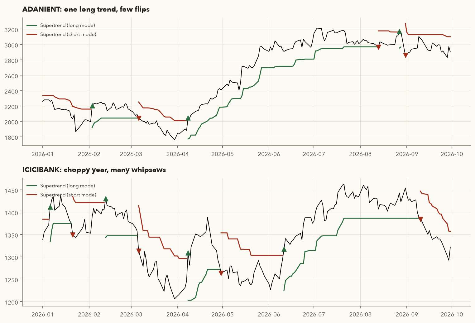
The same indicator, two very different years
| Stock | Long-only Supertrend trades in 2026 (entry → exit, close to close) | Sum |
|---|---|---|
| ADANIENT | 3 Feb 2,202.6 → 6 Mar 2,039.9 (−7.4%); 8 Apr 2,043.8 → 13 Aug 2,964.9 (+45.1%); 27 Aug 3,169.0 → 31 Aug 2,859.1 (−9.8%) | +27.9% |
| ICICIBANK | 6 Jan 1,411.2 → 21 Jan 1,349.0 (−4.4%); 12 Feb 1,430.0 → 6 Mar 1,313.4 (−8.2%); 8 Apr 1,309.2 → 30 Apr 1,263.4 (−3.5%); 11 Jun 1,317.0 → 10 Sep 1,384.5 (+5.1%) | −11.0% |
Supertrend gives fewer false signals than a simple price-vs-MA rule, as Varsity notes, but it cannot remove whipsaws in a stock that keeps reversing. Combine it with an ADX or 200-day filter, or use it purely as a trailing stop for trades you entered for other reasons.
13. Volume indicators: volume average, OBV, VWAP
13.1 Volume vs its 10-day average (Varsity's method)
Volume is the number of shares traded. A trade where one person buys 100 shares from another adds 100 to volume, not 200. Raw volume means little on its own, so Varsity compares today's volume with the average of the previous 10 sessions. Volume above that average suggests large participants ("smart money") are involved.
| Price | Volume vs 10-day avg | Varsity's reading |
|---|---|---|
| Up | Up | Bullish: real buying, likely institutions |
| Up | Down | Caution: weak buying, possible bull trap |
| Down | Up | Bearish: real selling |
| Down | Down | Caution: weak selling, possible bear trap |
The breakout that lacked volume, and the day that had it
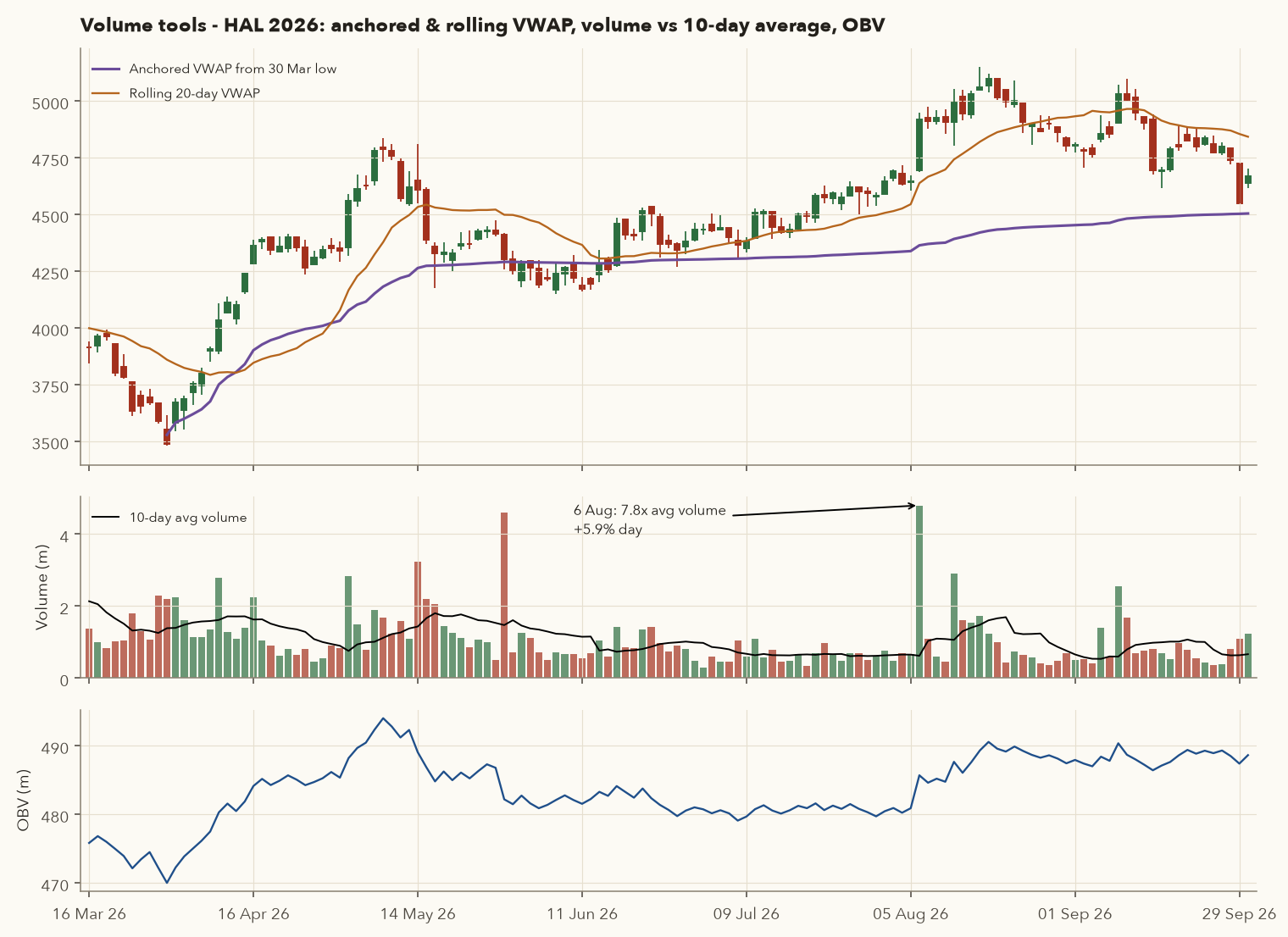
- 21 Jul 2026 (the Bollinger squeeze breakout, +2.02%): volume 697,566 vs 10-day average 642,844, a ratio of 1.09×. Only marginally above average, so this is a "price up, volume barely up" day and not a convincing breakout by Varsity's test.
- 6 Aug 2026 (+5.92%, close 4,920): volume 4,796,689 vs 10-day average 615,363, a ratio of 7.79×. This was the session that confirmed real demand, and HAL made its closing high of 5,099 on 18 Aug.
13.2 On-Balance Volume (OBV)
Joseph Granville's OBV keeps a running total. Add the day's volume on up-closes, subtract it on down-closes, and ignore flat days.
- \(OBV_t\)
- On-balance volume on day \(t\): a running total, counted in shares. \(OBV_{t-1}\) is yesterday's total.
- \(C_t - C_{t-1}\)
- Today's change in close: today's close minus the previous session's.
- \(\operatorname{sign}(\dots)\)
- +1 if the number inside is positive, −1 if it is negative, 0 if it is exactly zero.
- \(V_t\)
- Today's volume: the number of shares traded.
How it works: start the total anywhere (0 is fine). On an up-close add the day's volume, on a down-close subtract it, and on an unchanged close leave the total as it is. The HAL table below does this for six days.
The absolute level of OBV is meaningless. Only its direction matters. Rising OBV with rising price confirms the trend. Price making new highs while OBV does not is a volume divergence and a warning.
OBV step by step (rebased to 0 on 14 Jul)
| Date | Close | Volume | Direction | OBV |
|---|---|---|---|---|
| 14 Jul 2026 | 4,442.4 | 770,894 | – | 0 |
| 15 Jul | 4,420.5 | 440,343 | down → subtract | −440,343 |
| 16 Jul | 4,433.8 | 474,213 | up → add | 33,870 |
| 17 Jul | 4,500.7 | 658,032 | up → add | 691,902 |
| 20 Jul | 4,491.0 | 344,703 | down → subtract | 347,199 |
| 21 Jul | 4,581.7 | 697,566 | up → add | 1,044,765 |
Over the bigger picture, from 1 Apr to 30 Sep 2026 HAL's price rose 27.2% and OBV rose by 16.36 million shares. Volume confirmed the trend. Note also the May 2026 drop, where OBV fell sharply on heavy red-volume days (Figure 4.14), which is a "price down, volume up" warning in Varsity's table.
13.3 VWAP: intraday, rolling and anchored
Volume-Weighted Average Price is the average price paid per share, weighted by how many shares traded at each price. It answers the question "where is the average participant's cost?"
- \(H_t,\ L_t,\ C_t\)
- The high, low and close of bar \(t\), in ₹. A bar is one day on a daily chart, or one minute for intraday VWAP.
- \(TP_t\)
- The typical price of the bar: the average of its high, low and close. It stands in for "the price traded at" during that bar.
- \(V_t\)
- The volume (shares traded) in bar \(t\).
- \(\sum\)
- "Add up" over every bar in the window: since 9:15 am today for intraday VWAP, the last 20 days for a 20-day rolling VWAP, or every day since the chosen start date for anchored VWAP.
- \(VWAP\)
- The volume-weighted average price, in ₹.
- For each bar, compute the typical price and multiply it by the bar's volume. That is roughly the rupee value traded in the bar.
- Add those products up over the window, and separately add up the volumes.
- Divide the first total by the second. Heavy-volume bars pull VWAP towards their price more than quiet bars do. Price above VWAP means the average buyer in that window is in profit.
- Intraday VWAP (the version Varsity describes) restarts every day at 9:15 am. Price above VWAP means the intraday trend is up, and institutions judge their execution against it (a buy below VWAP is a "good fill"). It is an intraday tool. Since this course does not target intraday trading, you will mostly use the two variants below.
- Rolling VWAP (e.g., 20-day): the volume-weighted average over a moving window, roughly the average cost of everyone who bought in the last month. Price below it means the recent buyers are, on average, sitting on losses.
- Anchored VWAP (AVWAP): the cumulative VWAP starting from a chosen event, such as a major low, a breakout, or a results day. It shows the average cost of everyone who has bought since that event. In uptrends, pullbacks often hold near the AVWAP from the last major low.
Anchored VWAP from the 30 March 2026 low
| Date | High | Low | Close | Volume | TP | Cum TP×V (₹ cr) | Cum V | AVWAP |
|---|---|---|---|---|---|---|---|---|
| 30 Mar 2026 | 3,615.6 | 3,479.1 | 3,487.2 | 2,197,252 | 3,527.30 | 775.0 | 2,197,252 | 3,527.30 |
| 1 Apr | 3,688.6 | 3,545.0 | 3,670.8 | 2,246,768 | 3,634.80 | 1,591.7 | 4,444,020 | 3,581.65 |
| 2 Apr | 3,700.1 | 3,551.0 | 3,687.0 | 1,611,009 | 3,646.03 | 2,179.1 | 6,055,029 | 3,598.78 |
- 30 Mar: \(TP = (3{,}615.6 + 3{,}479.1 + 3{,}487.2)/3 = 3{,}527.30\). On the first day, AVWAP equals TP.
- 1 Apr: TP × V for the day is \(3{,}634.80 \times 2{,}246{,}768 = \text{₹}816.7\) crore, so the running total is \(775.0 + 816.7 = \text{₹}1{,}591.7\) crore (₹1,591.7 × 107). Divide by the running volume: \(AVWAP = 1{,}591.7 \times 10^7 / 4{,}444{,}020 = 3{,}581.65\).
- Since the anchor, HAL closed below its AVWAP on only 12 days, the last one on 16 Jun 2026, when the May–June pullback held near the line (about 4,290–4,300).
- On 30 Sep 2026: close 4,668.0, AVWAP 4,503.9 (buyers since the March low are still in profit on average), but the 20-day rolling VWAP was 4,842.5 (buyers in the last month are on average underwater). Long-term structure was intact, and short-term momentum was weak.
14. Donchian channels
Richard Donchian's channel is the simplest trend tool of all: the highest high and lowest low of the last n days. A close above the prior 20-day high is a breakout, and the famous "Turtle" traders of the 1980s used 20- and 55-day versions. It connects directly to Chapter 3's support and resistance. The channel is the most recent range.
- \(H,\ L\)
- Daily highs and lows, in ₹. \(H_{t-1}\) is yesterday's high and \(H_{t-n}\) the high \(n\) sessions ago.
- \(n\)
- The channel length in sessions: 20 for the entry channel, 10 for the exit line in the rule below.
- \(\max,\ \min\)
- The largest and the smallest value in the list.
- \(Upper_t,\ Lower_t\)
- The highest high and lowest low of the previous \(n\) sessions. Today is not included.
- \(Mid\)
- The midpoint of the channel.
How it works: look back over the last \(n\) sessions, not counting today, and note the highest high and the lowest low. A close above \(Upper_t\) is an upside breakout. A close below \(Lower_t\) is a downside break.
Example (TITAN, 16 Jun 2026, \(n = 20\)): the 20 sessions from 18 May to 15 Jun had a highest high of 4,297.0 (15 Jun) and a lowest low of 3,962.8 (11 Jun). So \(Upper = 4{,}297.0\), \(Lower = 3{,}962.8\) and \(Mid = 4{,}129.9\). TITAN closed at 4,338.0 on 16 Jun, above 4,297.0. That is the last breakout entry in the table below.
(We use the previous n days, so today's close can break the channel.) A classic swing rule is: buy on a close above the 20-day high, and exit on a close below the 10-day low.
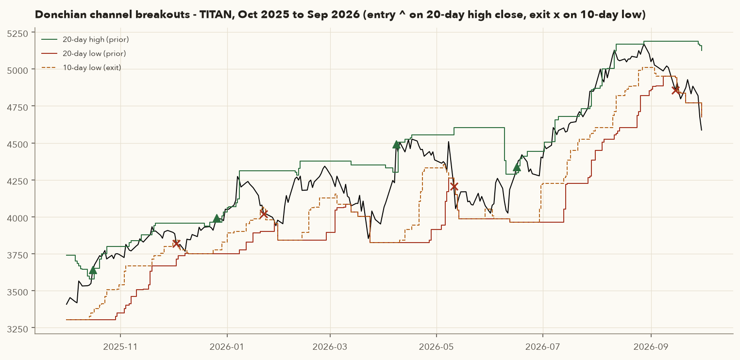
20-day breakout / 10-day low exit on a steady uptrend
| Entry | Price | Exit | Price | Result |
|---|---|---|---|---|
| 11 Apr 2025 | 3,234.9 | 12 Jun 2025 | 3,452.7 | +6.7% |
| 25 Jun 2025 | 3,652.2 | 8 Jul 2025 | 3,441.3 | −5.8% |
| 18 Aug 2025 | 3,554.8 | 12 Sep 2025 | 3,571.9 | +0.5% |
| 16 Oct 2025 | 3,640.3 | 3 Dec 2025 | 3,817.8 | +4.9% |
| 26 Dec 2025 | 3,992.0 | 22 Jan 2026 | 4,018.6 | +0.7% |
| 8 Apr 2026 | 4,492.5 | 11 May 2026 | 4,205.6 | −6.4% |
| 16 Jun 2026 | 4,338.0 | 15 Sep 2026 | 4,856.0 | +11.9% |
7 trades, 5 winners, sum +12.5% (average win +4.9%, average loss −6.1%). Buying and holding TITAN returned +53.6% from 1 Apr 2025 to 30 Sep 2026 (+41.8% even if you started on the first entry day, 11 Apr 2025). TITAN rose steadily with frequent sharp dips, so a tight 10-day exit kept shaking the system out. Two lessons follow. The channel lengths must fit the stock's rhythm (a 20/55 or ATR-based exit would have held longer). And trend-following systems earn their keep across many stocks, not on one chart (Chapter 12).
15. Relative strength vs Nifty (RS line and Mansfield RS)
For stock selection, this may be the most useful tool in the chapter. The question is not "is this stock going up?" but "is it going up more than the market?" Leadership tends to persist for months (the momentum effect, documented in many markets, including India). Stocks that outperform in a weak market are often the first to run when the market turns.
- \(C^{stock}_t\)
- The stock's close in week \(t\), in ₹ (we use the last close of each week).
- \(C^{Nifty}_t\)
- Nifty 50's close on the same date, in index points.
- \(RS_t\)
- The RS line: stock price divided by Nifty. Its level means nothing on its own. Only its direction matters: rising = the stock is beating Nifty.
- \(SMA_{52\,weeks}(RS)_t\)
- The average of the last 52 weekly RS values: the stock's one-year "normal" relationship with Nifty.
- \(\text{Mansfield RS}_t\)
- How far this week's RS is above (+) or below (−) that one-year average, in %.
- Divide the stock's weekly close by Nifty's weekly close. That is the RS line.
- Average the last 52 weekly RS values.
- Divide this week's RS by that average, subtract 1 and multiply by 100. Above zero means the stock is doing better against Nifty than it usually does. The paragraph below explains the zero-line cross.
The RS line rises when the stock outperforms Nifty, even if both are falling. Mansfield RS (named after the Mansfield chart service and popularised by Stan Weinstein, using weekly data) compares the RS line with its own 52-week average. Above zero means the stock is outperforming its normal relationship with the index. Crossing from negative to positive is a classic early leadership signal.
Mansfield RS by hand
- \(RS = 4{,}587.0 / 22{,}620.45 = 0.20278\).
- Average of the weekly RS over the last 52 weeks: 0.1753.
- \(\text{Mansfield} = (0.20278/0.1753 - 1) \times 100 = +15.7\). TITAN was 15.7% stronger relative to Nifty than its one-year norm.
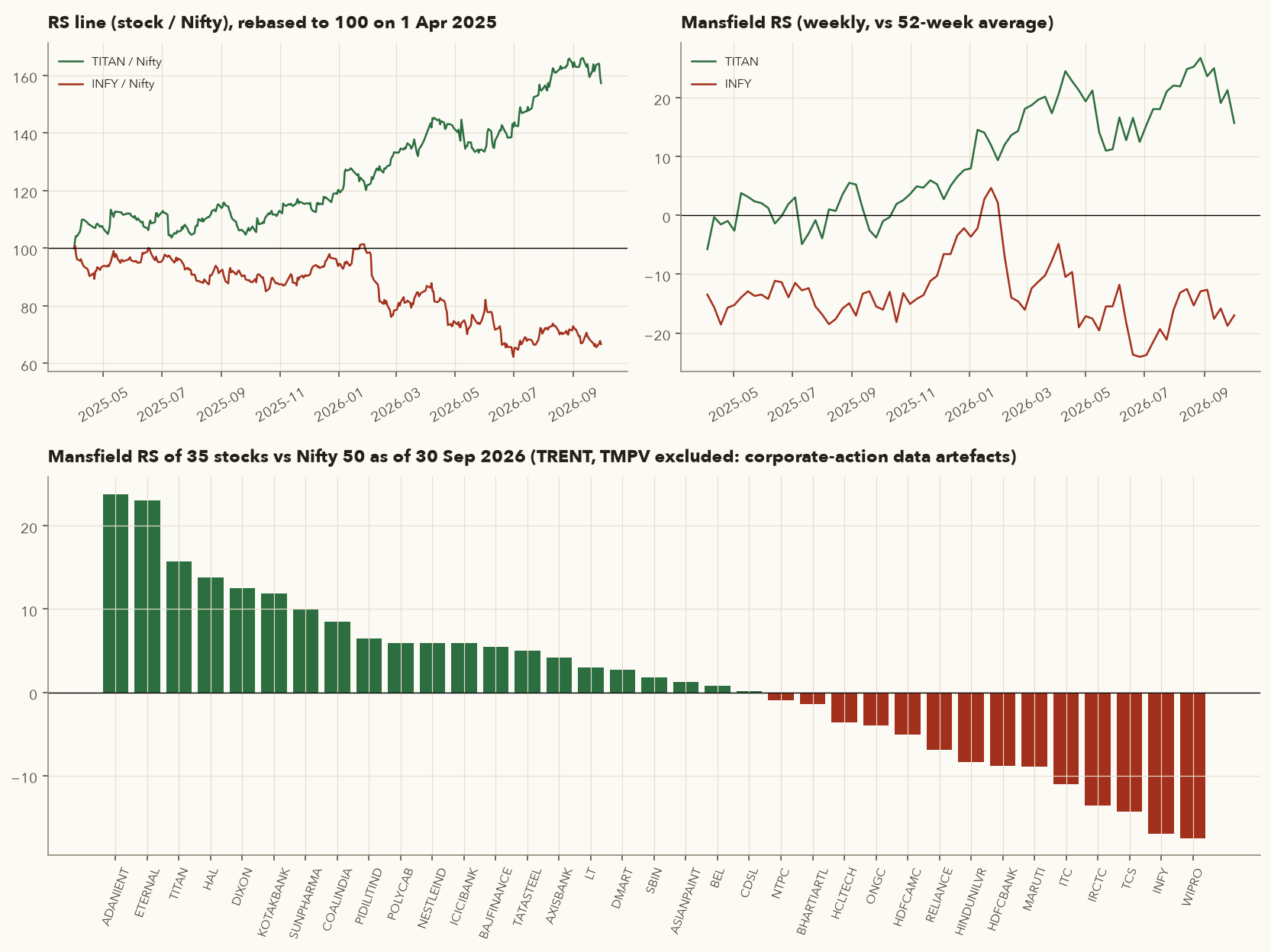
| Leaders (30 Sep 2026) | Mansfield RS | 6-month return | Laggards | Mansfield RS | 6-month return |
|---|---|---|---|---|---|
| ADANIENT | +23.8 | +65.1% | WIPRO | −17.5 | −15.5% |
| ETERNAL | +23.1 | +39.8% | INFY | −17.0 | −20.5% |
| TITAN | +15.7 | +16.1% | TCS | −14.3 | −13.1% |
| HAL | +13.8 | +33.9% | IRCTC | −13.6 | −7.9% |
| DIXON | +12.5 | +35.4% | ITC | −11.0 | −8.7% |
Over the same six months (31 Mar – 30 Sep 2026), Nifty returned +1.3%. Notice how the IT sector (WIPRO, INFY, TCS, HCLTECH) clusters at the bottom. RS ranking reveals sector rotation without reading a single news article. Also notice that ETERNAL, HAL and DIXON were rising in RS (from +2.4, +2.6 and −4.8 thirteen weeks earlier), while ADANIENT's was falling from +37.5. Both the level and the direction matter.
RS is backward-looking, and leaders can reverse sharply (DIXON was −19.7% over the year to 30 Sep 2026 despite its recent strength). Use RS to build a shortlist, then apply your trend, entry and risk rules. Corporate actions (splits, bonuses, demergers) can corrupt the RS line if the data is not adjusted, which is why TRENT and TMPV are excluded here.
16. Other indicators in Varsity's list
Varsity's "Other indicators" chapter covers a few more tools. You should recognise them, but none adds a new kind of information beyond the families above.
| Indicator | Construction (default) | How it is read | Family |
|---|---|---|---|
| Alligator (Bill Williams) | Three offset SMAs: jaw 13, teeth 8, lips 5 | Lines fanned out in order (price > 5 > 8 > 13) = trend; tangled lines = no trade | Trend (MA stack) |
| Aroon (Tushar Chande) | Days since the 25-day high / low, scaled 0–100 | Aroon-Up > 50 and Aroon-Down < 30 = uptrend (and vice versa); oscillator = Up − Down | Trend (time-based) |
| ATR bands | MA ± ATR | A close outside the band suggests continuation in that direction | Volatility envelope |
| Central Pivot Range | From the previous day's H, L, C: Pivot = (H+L+C)/3, BC = (H+L)/2, TC = 2 × Pivot − BC | Intraday support/resistance; Varsity has a separate chapter | Intraday levels |
17. Context test: the same RSI signal across 37 stocks
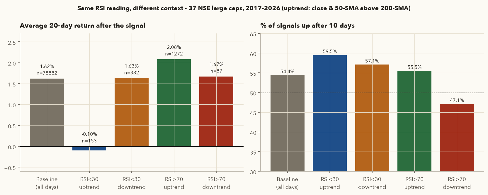
Books often state that "RSI below 30 is a buy in an uptrend but a trap in a downtrend". Instead of taking that on faith, we tested it on the 37 stocks in our data, 2017–2026.
- Signals: the day RSI(14) crosses below 30 ("oversold"), and the day it crosses above 70 ("overbought").
- Context: uptrend = close above the 200-day SMA and 50-day SMA above the 200-day SMA. Downtrend = both below.
- Outcome: the return over the next 10 and 20 trading days. Windows touching corporate-action artefacts (CDSL listing, TMPV demerger, TRENT bonus) were excluded. No costs.
| Case | Signals | Avg 10-day | % up at 10 days | Avg 20-day | Median 20-day | Worst 10% (20-day) |
|---|---|---|---|---|---|---|
| All stock-days (baseline) | 78,882 | +0.81% | 54.4% | +1.62% | +1.14% | −8.2% |
| RSI < 30, any trend | 877 | +0.56% | 56.1% | +0.89% | +0.93% | −10.9% |
| RSI < 30 in uptrend | 153 | −0.30% | 59.5% | −0.10% | +0.83% | −11.1% |
| RSI < 30 in downtrend | 382 | +1.41% | 57.1% | +1.63% | +0.94% | −9.7% |
| RSI > 70, any trend | 1,682 | +1.13% | 56.1% | +2.14% | +1.36% | −7.4% |
| RSI > 70 in uptrend | 1,272 | +1.05% | 55.5% | +2.08% | +1.23% | −7.7% |
| RSI > 70 in downtrend | 87 | +0.45% | 47.1% | +1.67% | +0.63% | −8.0% |
| Average 20-day return by period | RSI<30 uptrend | RSI<30 downtrend | RSI>70 uptrend | RSI>70 downtrend | Baseline |
|---|---|---|---|---|---|
| 2017–2019 | +2.48% (n=43) | +1.64% (99) | +0.40% (299) | −1.40% (15) | +1.31% |
| 2020–2022 | −1.10% (39) | +0.28% (106) | +3.21% (472) | +3.19% (37) | +2.26% |
| 2023–2026 | −1.12% (71) | +2.43% (177) | +2.02% (501) | +1.39% (35) | +1.29% |
- Context changes the result a lot. The same "RSI < 30" reading produced −0.10% or +1.63% average 20-day returns depending on the trend, and the ranking flipped between 2017–19 and 2020–26. A rule that worked in one period failed in the next.
- The textbook claim did not hold in this sample. Oversold readings in uptrends were rare (153 in 9 years across 37 stocks) and, after 20 days, did slightly worse than average, even though 59.5% were up after 10 days. When a large cap in a strong uptrend suddenly becomes deeply oversold, something real (results, a regulatory event) has often happened. Large-cap downtrends, by contrast, often saw sharp relief bounces.
- "Overbought" was not bearish. RSI > 70 in an uptrend was followed by the best average 20-day return of all the groups (+2.08% vs +1.62% baseline), which supports Varsity's point that sustained overbought readings show strength. In downtrends, the 10-day hit rate fell to 47.1%.
- No signal here is a system. The differences are a few tenths of a percent and the worst-decile outcomes (−7% to −11%) dwarf them. An RSI threshold alone gives you no edge worth trading. The value comes from combining a regime filter, an entry trigger, an ATR-based stop and position sizing, and then testing the whole package (Chapter 12).
18. Combining indicators without redundancy
18.1 Most oscillators measure the same thing
Beginners often pile RSI, Stochastic, CCI, Williams %R and MACD onto one chart and feel reassured when they "all agree". They agree because they are built from the same closes over similar windows. Here is the correlation of daily readings across all 37 stocks since 2018:
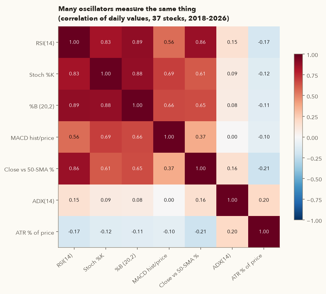
- RSI vs %B: 0.89. RSI vs Stochastic: 0.83. RSI vs distance from 50-SMA: 0.86. Three momentum readings that are close to one reading.
- ADX vs RSI: 0.15. ATR% vs RSI: −0.17. These answer genuinely different questions (trend strength, volatility).
18.2 One trend + one momentum + one volatility tool
| Job | Question it answers | Pick ONE |
|---|---|---|
| Trend / regime | Should I be looking for longs, shorts, or nothing? | 200-SMA (with 50-SMA), or ADX/DMI, or Supertrend |
| Momentum / timing | Is this a good moment to enter (pullback ending, breakout starting)? | RSI, or MACD, or Stochastic |
| Volatility / risk | Where is my stop, and how big can my position be? | ATR (Bollinger bandwidth if you trade squeezes) |
| Optional: participation | Is real money behind the move? | Volume vs 10-day average, or OBV |
| Optional: selection | Which stocks to look at in the first place? | Relative strength vs Nifty |
Varsity puts indicators last in its decision hierarchy: (1) a recognisable candlestick pattern, (2) support/resistance for entry and stop, (3) volume above average, and only then (4) indicator confirmation. If the indicators agree, take the full position. If they don't, trade smaller or skip, but do not reject an otherwise valid setup just because of an indicator, and do not take a trade on an indicator alone.
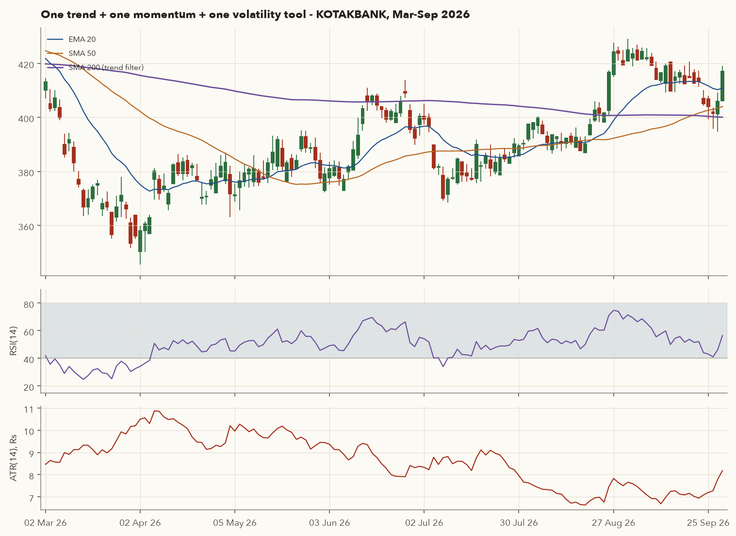
Reading a chart with three non-overlapping tools
- Trend: close ₹417.0 above the 200-SMA (400.1). The 50-SMA (404.0) crossed above the 200-SMA on 22 Sep 2026, a fresh golden cross. ADX 28.3 with +DI 23.3 > −DI 18.6, so a trend is present and up. Mansfield RS +11.9 (outperforming Nifty, which was 7.2% below its 200-SMA).
- Momentum: during the September pullback RSI dipped to 40.99 on 28 Sep, right at the floor of the uptrend 40–80 band, and recovered to 56.5 by 30 Sep. That is the "uptrend oversold" reading from Section 6.4.
- Volatility/risk: ATR ₹8.18 (1.96% of price). A 2×ATR stop sits at \(417.0 - 16.36 = \text{₹}400.64\), right next to the 200-SMA. Two independent reasons support the same level, which is the kind of confluence you look for.
- Sizing (₹5,00,000 account, 1% risk): \(\lfloor 5{,}000/16.36 \rfloor = 305\) shares, about ₹1,27,185 (25.4% of capital), risk ₹4,991.
- What could go wrong: the broad market was in a downtrend (Nifty death cross since March), golden crosses are slow and often fail (Section 4), and Section 17 showed that no single reading is an edge. A disciplined trader would also check the candlestick trigger, support/resistance and volume (Chapters 2–3), and what's coming up (results, events) before acting.
Every indicator here works on any timeframe. For positional trades and investments, compute them on weekly bars (a 10-week SMA ≈ 50-day, a 40-week SMA ≈ 200-day, weekly RSI 14), and use the daily chart only to time the entry. A clean multi-timeframe rule is to trade in the direction of the weekly trend and enter on a daily pullback.
The course framework (framework/, built in Chapter 17) implements every indicator in this chapter in framework.indicators: sma, ema, rsi (Wilder), macd, bollinger, stochastic, atr (Wilder), adx, obv, vwap_rolling, supertrend, donchian, relative_strength(df, bench_df), mansfield_rs(df, bench_df) (this chapter's weekly version, 52-week average) and pivots (swing highs/lows). ATR-based sizing lives in framework.risk.position_size(capital, risk_pct, entry, stop, lot_size=1) framework.risk.atr_stop and framework.risk.chandelier_stop. The swing scanner python -m framework.scan combines a 200/50-SMA trend filter, an RSI pullback trigger (RSI dipped below 45) and an ATR-based stop, the same three-job structure as this section. The EMA and Wilder averages are seeded with a simple average exactly as in this chapter, so the framework reproduces its numbers.
19. Try it yourself
These snippets need a copy of the course repository and Python with pandas and numpy (setup steps are in its framework/README.md). Run them from the repository's root folder, for example with .venv/bin/python, because the file paths are relative to that folder. Each snippet is self-contained and reproduces numbers from this chapter.
19.1 SMA, EMA and Wilder RSI on SBIN
import pandas as pd

def load(sym):
    df = pd.read_csv(f"data/ohlc/{sym}.csv", index_col=0, parse_dates=True)
    return df[~((df.Volume == 0) & (df.High == df.Low))]   # drop holiday placeholder bars

def wilder(s, n):
    # seed with the simple mean of the first n values, then (prev*(n-1) + x) / n
    s = s.dropna(); out = pd.Series(index=s.index, dtype=float)
    out.iloc[n-1] = s.iloc[:n].mean()
    for i in range(n, len(s)):
        out.iloc[i] = (out.iloc[i-1]*(n-1) + s.iloc[i]) / n
    return out

df = load("SBIN")
c = df.Close
sma20 = c.rolling(20).mean()
ema20 = c.ewm(span=20, adjust=False).mean()     # alpha = 2/(20+1)
d = c.diff()
avg_gain = wilder(d.clip(lower=0), 14)
avg_loss = wilder((-d).clip(lower=0), 14)
rsi14 = 100 - 100 / (1 + avg_gain / avg_loss)
print(pd.DataFrame({"close": c, "sma20": sma20, "ema20": ema20, "rsi14": rsi14}).tail(3).round(2))
# 2026-09-30: close 959.5, sma20 992.47, ema20 992.55, rsi14 33.72
19.2 MACD, Bollinger %B, ATR and position size on HAL
import pandas as pd
df = pd.read_csv("data/ohlc/HAL.csv", index_col=0, parse_dates=True)
df = df[~((df.Volume == 0) & (df.High == df.Low))]
c = df.Close
macd = c.ewm(span=12, adjust=False).mean() - c.ewm(span=26, adjust=False).mean()
signal = macd.ewm(span=9, adjust=False).mean()
mid = c.rolling(20).mean(); sd = c.rolling(20).std(ddof=0)
upper, lower = mid + 2*sd, mid - 2*sd
pct_b = (c - lower) / (upper - lower)
prev = c.shift(1)
tr = pd.concat([df.High - df.Low, (df.High - prev).abs(), (df.Low - prev).abs()], axis=1).max(axis=1)
atr14 = tr.ewm(alpha=1/14, adjust=False).mean()          # Wilder smoothing
day = "2026-07-21"
print(round(pct_b[day], 3), round(atr14[day], 2))        # 1.097 95.92
entry, stop = c[day], c[day] - 2*atr14[day]
print("qty for 1% of Rs 5 lakh:", int(5000 // (entry - stop)))   # 26
19.3 Rank stocks by Mansfield relative strength
import pandas as pd, glob, os
nifty = pd.read_csv("data/ohlc/IDX_NSEI.csv", index_col=0, parse_dates=True).Close
rows = []
for f in glob.glob("data/ohlc/*.csv"):
    sym = os.path.basename(f)[:-4]
    if sym.startswith("IDX_") or sym in ("TRENT", "TMPV"):   # skip indices and adjustment artefacts
        continue
    c = pd.read_csv(f, index_col=0, parse_dates=True).Close
    rs = (c / nifty.reindex(c.index).ffill()).resample("W-FRI").last().dropna()
    mansfield = (rs / rs.rolling(52).mean() - 1) * 100
    rows.append((sym, round(mansfield.iloc[-1], 1)))
print(sorted(rows, key=lambda r: -r[1])[:5])
# [('ADANIENT', 23.8), ('ETERNAL', 23.1), ('TITAN', 15.7), ('HAL', 13.8), ('DIXON', 12.5)]
Exercises with code: (a) change the RSI lookback to 7 and to 21 and count how many days SBIN spent above 70 in 2025–26; (b) rerun the Section 17 test with a 2-day RSI below 10 (the full script is course/scripts/ch04_figures.py, function context_test); (c) compute the Supertrend on your own favourite stock with multipliers 2, 3 and 4 and count the flips.
20. Practical checklist
- I identified the regime first: price vs 200-SMA (and 50 vs 200), ADX above or below 20–25, and the Nifty's own regime.
- I am using a tool that suits that regime: trend tools (MA, Supertrend, Donchian, MACD) in trends, range tools (Bollinger fades, Stochastic, RSI 30/70) only when ADX is low and bands are flat.
- I use at most one indicator per job: trend, momentum, volatility (plus optional volume and RS). No three oscillators saying the same thing.
- In uptrends I read RSI in the 40–80 frame (40–45 = pullback zone). In downtrends, in the 20–60 frame.
- I treat divergences and squeezes as alerts, and I wait for price confirmation (a higher low, a breakout close, volume).
- Breakouts: volume is above the 10-day average (ideally 1.5× or more). If not, I trade smaller or skip.
- My stop is based on structure and at least 1–2 × ATR away from entry. My position size = risk budget ÷ (entry − stop).
- For futures, I checked that (stop distance × lot size) fits within my per-trade risk. If not, I don't trade.
- I shortlisted stocks with positive and rising relative strength vs Nifty.
- I used the weekly chart for the big picture and the daily chart for timing.
- I have not tuned settings to fit one chart. Any rule I rely on has been tested across many stocks and periods, net of costs (Chapter 12).
- I know my indicator values may differ slightly from my broker's chart, and that is fine.
21. Key takeaways
- Indicators are transformations of price and volume. They organise information. They do not add new information or predict the future.
- Four families do four different jobs: trend (MAs, MACD, ADX, Supertrend, Donchian), momentum (RSI, Stochastic, MACD histogram), volatility (ATR, Bollinger bandwidth) and volume (volume average, OBV, VWAP). Relative strength is a fifth, for selection.
- Trend tools win in trends and bleed in ranges. Oscillators do the opposite. Identify the regime first.
- EMA uses \(\alpha = 2/(n+1)\). Wilder's RSI, ATR and ADX use \(\alpha = 1/n\), so they have long memories, and charting platforms compute them over the full history.
- The Nifty 50/200 golden cross was a poor timing tool in 2017–2026 (2 of 6 profitable, system CAGR 2.8% vs 9.3% buy-and-hold). Use it as a regime label, not a trigger.
- RSI ranges shift with trend (40–80 up, 20–60 down). "Overbought" in an uptrend was bullish in our 37-stock test. "Oversold" can persist for weeks (Nifty, Sep 2026), and the textbook "buy oversold only in uptrends" rule did not hold in our data.
- Bollinger squeezes predict bigger moves, not direction (53% follow-through in 86 cases). Band walks punish mean-reversion shorts in trends.
- ATR is the most practical indicator. Use it for stops (1.5–3 × ATR), chandelier trailing exits, comparing volatility across stocks, and checking whether a futures lot fits your risk budget.
- RSI, Stochastic and %B correlate 0.83–0.89. Use one per job: one trend + one momentum + one volatility tool.
- Test every rule across many stocks and periods. In our data, the textbook RSI-in-uptrend claim did not hold, and results flipped between periods.
22. Quiz and exercises
Q1. A stock's 20-day EMA yesterday was ₹500. Today it closes at ₹521. What is today's 20-day EMA?
Q2. Yesterday's Wilder averages were: average gain 3.00, average loss 1.50 (14-period). Today the stock falls by 6.00. What were yesterday's and today's RSI?
Today: gain = 0, loss = 6.00. \(\overline G = (3.00 \times 13 + 0)/14 = 2.786\); \(\overline L = (1.50 \times 13 + 6.00)/14 = 1.821\); \(RS = 1.530\); \(RSI = 100 - 100/2.530 = 60.47\). One sharp down day cost about 6 RSI points.
Q3. Yesterday a stock closed at ₹500. Today it gapped up and traded between ₹520 and ₹530. What is today's true range, and why not just use high − low?
Q4. You have ₹3,00,000 and risk 1% per trade. Entry is ₹1,200, ATR(14) is ₹30, and you use a 2×ATR stop. How many shares can you buy, and what percentage of capital is the position?
Q5. A stock's 20-day SMA is ₹1,000 and the 20-day SD is ₹25. It closes at ₹1,040. Compute the Bollinger Bands, %B and bandwidth.
Q6. The 12-day EMA is 520, the 26-day EMA is 510 and the signal line is 12. Read the MACD.
Q7. Nifty's golden cross on 11 Nov 2019 was followed by a −30.6% move before the next death cross. What does this teach about crossovers?
Q8. A stock has ADX 15, with +DI 22 above −DI 18. A friend says "+DI is above −DI, so it's an uptrend, buy." What do you say?
Q9. Your chart shows RSI(14), Stochastic(14,3,3) and Bollinger %B all "oversold". Why is this weaker confirmation than it looks, and what would you replace two of them with?
Q10. A stock's price/Nifty ratio today is 0.25, and its 52-week average of that ratio is 0.20. What is its Mansfield RS, and what does it mean if the stock fell 5% this month?
Q11. You have ₹10,00,000, risk 1% per trade, and want to trade one HAL futures lot (150 shares) with a 2×ATR stop of ₹191.83 per share. Is it allowed under your rule? What are your options?
Q12. ADANIENT touched its upper Bollinger Band on 13 Apr 2026 (%B ≈ 1.00). Varsity's mean-reversion rule says short with a target at the middle band. Why did this fail, and what would have warned you?
Q13. Starting from OBV = 0, a stock closes 100 → 102 (volume 50,000) → 101 (30,000) → 104 (80,000). What is OBV after each day? The 10-day average volume is 40,000. How does Varsity's volume table read the last day?
Q14. You are long and Supertrend (10,3) is in long mode with yesterday's line (final lower band) at ₹1,820. Today's basic lower band works out to ₹1,805 and the stock closes at ₹1,850. What is today's Supertrend line, and why?
Q15 (exercise). Using the try-it code, compute RSI(14) for INFY and count how many sessions from Oct 2025 to Sep 2026 it spent below 30 and above 70. Does the result fit the "downtrend: 20–60" idea?
23. Sources
Primary (concepts, explained here in our own words):
Zerodha Varsity, Module 2, Ch 12: Volumes ·
Ch 13: Moving Averages ·
Ch 14: Indicators (Part 1) — momentum, RSI, leading vs lagging ·
Ch 15: Indicators (Part 2) — MACD, Bollinger Bands, avoiding indicator overload ·
Ch 20: Other indicators — ADX, Alligator, Aroon, ATR, ATR bands, Supertrend, VWAP ·
Ch 22: The Central Pivot Range ·
Module 2 index.
Original indicator definitions: J. Welles Wilder, New Concepts in Technical Trading Systems (1978) for RSI, ATR, ADX/DMI and Wilder smoothing; Gerald Appel (MACD); John Bollinger, Bollinger on Bollinger Bands (2001) for %B, bandwidth, squeeze and band walk; George Lane (Stochastic); Joseph Granville (OBV); Richard Donchian (channels); Stan Weinstein, Secrets for Profiting in Bull and Bear Markets (1988) for Mansfield relative strength. Supertrend defaults: Kite (7,3) as stated in Varsity Ch 20; TradingView built-in (10,3).
Data: NSE daily OHLCV via Yahoo Finance (course dataset, snapshot to 30 Sep 2026; zero-volume holiday placeholder bars removed); NSE F&O UDiFF bhavcopy 30 Sep 2026 for the HAL futures lot size (150). All figures and numbers are reproducible with course/scripts/ch04_figures.py (indicator code in course/scripts/ch04_indicators.py).