
Swing Trading Playbook
1. What you'll learn and why it matters
Chapters 2 to 4 gave you the parts: candlesticks, support and resistance, trends, chart patterns, moving averages, RSI, ATR and volume. This chapter puts the parts together into a playbook: a written process you can follow every evening, in about 30 to 60 minutes, without watching the screen during market hours.
By the end you will be able to:
- Decide, from three numbers, whether the market is friendly to new long trades (the regime).
- Pick strong sectors and strong, liquid stocks (relative strength).
- Trade four concrete setups with exact rules for entry, stop, size and exit.
- Size every position so that one loss costs about 1% of your account.
- Manage trades with partial profits, breakeven stops, trailing stops and time stops.
- Place the orders with GTT (Good Till Triggered) so you don't need to watch prices all day.
- Keep a trade journal, run a weekly review and judge a setup by its numbers, not by memory.
Swing trader: this is your core manual. Positional trader: Setup 4 (weekly trend + daily trigger) and the trailing rules let you hold for months. Long-term investor: the regime and relative-strength gates are a useful timing layer on top of the fundamental work in Chapters 6 to 8. Future futures trader: the same process applies to stock futures in Chapter 9, but leverage makes the sizing and gap-risk sections far more important.
Every number below comes from historical NSE data, computed with Python. The examples are historical analysis, not recommendations. The backtests include losers, and in 2025-26 three of the four setups lost money on our stock list. Trading involves real risk of loss. Treat this chapter as a way to build judgement, not as a promise of returns.
2. What swing trading is (and isn't)
Swing trading means holding a position for a few days to a few weeks to capture one "swing": one leg of a trend, or a bounce from a level. Varsity's Module 2 finale also calls this positional trading and recommends it to beginners over day trading, because you decide with end-of-day (EOD) data, calmly, after the close.
| Style | Typical hold | Chart used | Screen time | Main risk |
|---|---|---|---|---|
| Intraday / scalping | Minutes to hours | 1-15 min | All day | Costs, noise, emotions |
| Swing | 2 days to ~6 weeks | Daily (with weekly for context) | 30-60 min each evening | Overnight gaps, events |
| Positional / trend | 1-6 months | Weekly + daily | ~1 hour a week + checks | Giving back open profit |
| Investing | Years | Fundamentals; monthly/weekly charts | Quarterly reviews | Business and valuation risk |
The practical frame (from Varsity, adapted)
- Timeframe: daily candles (EOD). The higher the timeframe, the more reliable a signal tends to be.
- Lookback: look at 6 to 12 months of daily candles when judging a setup. Extend to about 2 years when you mark support and resistance.
- Opportunity universe: don't scan 2,000 stocks. Build a fixed list of liquid names you know. Varsity suggests the Nifty 50 as a starting universe, or a minimum volume of around 5 lakh shares a day. This course uses a 37-stock list of large, liquid NSE names.
- Time commitment: one focused evening session (Section 17) plus a weekly review on the weekend (Section 16).
What it costs, and how it is taxed (briefly)
Swing trades are delivery trades (product type CNC on Zerodha): you buy, the shares reach your demat account and you sell days later. As of Zerodha's published charges (checked October 2026), equity delivery has zero brokerage, but statutory charges still apply: STT (Securities Transaction Tax) 0.1% on both buy and sell, NSE transaction charges 0.00307%, SEBI fee Rs 10 per crore, GST 18% on (transaction + SEBI charges), stamp duty 0.015% on the buy side, and a DP charge of Rs 15.34 per stock per day on which you sell. On a Rs 1.1-1.25 lakh position, the worked examples in this chapter come to 0.23-0.26% of the buy value for the round trip: STT alone is 0.2%, and two partial sells mean two DP charges. The backtests use a flat 0.24%. Section 9 works out one example line by line.
Gains on listed shares held 12 months or less are short-term capital gains, taxed at 20% plus cess for FY 2026-27 (unchanged since 23 July 2024). Very frequent trading can also raise the question of whether your income is business income. Chapter 13 covers costs and tax in detail. In this chapter, costs are included in every R-multiple (the profit or loss of a trade measured in units of its initial risk, defined in Section 7). Taxes are not.
3. The top-down process in one picture
A professional swing trader doesn't start with a hot stock. They start with the market and narrow down. Every trade must pass eight gates, in order:
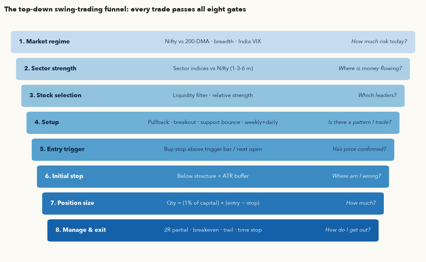
The logic: most stocks move with the market most of the time. Varsity's Dow Theory chapters make the same point with the primary trend: fighting it lowers your odds. So the first question is "is the tide coming in?" Then "which boats are rising fastest?" (sectors and relative strength). Only then "is there a low-risk place to step on board?" (the setup, trigger and stop). Finally, "how big, and how do I get off?" (size and management).
Varsity's finale chapter describes a two-part daily routine. Part 1, shortlisting: flip through every chart in your universe and look only at the last 3-4 candles for a recognisable pattern. Part 2, evaluation: spend 15-20 minutes on each of the 4-5 shortlisted charts and check them against a strict checklist. Usually only 1-2 qualify, and on some days none do. Deciding not to trade is a trading decision too. Our playbook adds the regime and sector gates in front of that routine.
4. Gate 1: market regime
The regime answers one question: how much risk should I take on new long trades today? We use three measures, all computed from end-of-day data.
4.1 Nifty 50 versus its 200-day moving average
Plain language: the 200-day simple moving average (200-DMA) is the average closing price of the last ~10 months. If the index is above it, and the average itself is rising, the long-term trend is up.
The logic: the 200-DMA is a slow, widely watched line. When price is above it, the average investor who bought in the last 10 months is in profit, so dips tend to get bought. Below it, rallies tend to get sold by people who want to get out at breakeven. It does not predict tomorrow. It describes the "weather".
- \(C_t\)
- Nifty 50's close on day \(t\) (today), in index points. \(C_{t-k}\) is the close \(k\) sessions ago.
- \(\textstyle\sum_{k=0}^{199}\)
- "Add up" the terms for \(k = 0\) (today) to \(k = 199\): the last 200 closes.
- \(\text{SMA}_{200,t}\)
- The 200-day simple moving average (200-DMA) on day \(t\): the plain average of those 200 closes.
- \(\text{Distance}\)
- How far today's close is above (+) or below (−) the 200-DMA, in %.
How it works: add the last 200 closes and divide by 200. Then divide today's close by that average, subtract 1 and multiply by 100. A positive distance means Nifty is above its long-term average. For the slope, compare today's 200-DMA with its value 20 sessions earlier: higher means rising.
Where is the market versus its 200-DMA?
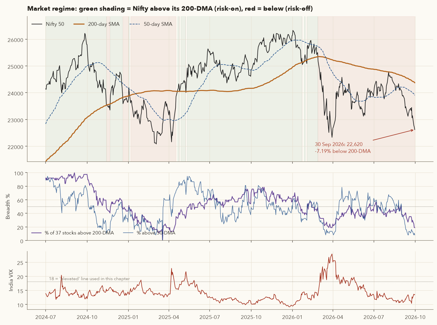
- Nifty close on 30 Sep 2026: \(C_t = 22{,}620.45\).
- Average of the last 200 closes: \(\text{SMA}_{200} = 24{,}372.85\).
- Distance = \((22{,}620.45 / 24{,}372.85 - 1) \times 100 = -7.19\%\).
- Slope: the 200-DMA is 1.09% lower than it was 20 sessions earlier, so it is falling.
- Verdict: price below a falling 200-DMA. Nifty last crossed below it on 27 Feb 2026 and has stayed below since, through the March 2026 sell-off (VIX peaked at 27.89 on 30 Mar 2026). Risk-off.
4.2 Breadth: how many stocks are participating?
An index can be held up by a handful of giants while most stocks fall. Breadth counts how many stocks in your universe are above their own moving averages.
- \(\#\{\dots\}\)
- "The number of" things described inside the braces.
- \(C\)
- Each stock's latest close, in Rs.
- \(\text{SMA}_{200}\)
- That stock's own 200-day simple moving average.
- \(\text{Breadth}_{200}\)
- The share of stocks in your universe that close above their own 200-DMA, in %.
How it works: for each stock in your universe, check whether today's close is above its 200-day average. Count the yeses, divide by the number of stocks with at least 200 days of history, and multiply by 100. Above 50% means most stocks are in long-term uptrends. The same calculation with the 50-day average gives breadth50.
On 30 Sep 2026 only 7 of 37 stocks (18.9%) were above their 200-DMA, and only 3 of 37 (8.1%) were above their 50-DMA. That is a very weak tape. When fewer than 1 in 5 stocks are in a long-term uptrend, buying setups have little tailwind.
4.3 India VIX: the market's fear gauge
India VIX is computed by NSE from Nifty option prices. It estimates the annualised volatility the market expects over the next 30 days. Roughly, a VIX of 13 implies typical daily Nifty moves of about \(13/\sqrt{252} \approx 0.8\%\). On 30 Sep 2026 VIX was 13.49, close to its 1-year median of 12.6. So the current weakness is a slow grind, not a panic. In March 2026 VIX hit 27.89, and daily swings and overnight gaps were much larger.
How we use VIX: not as a buy or sell signal, but as a size dial. Higher VIX means wider stops and more gap risk. Because our stops are ATR-based, a volatile market automatically gives smaller share counts. On top of that, many traders halve their per-trade risk when VIX is above ~18.
| Date | Nifty | 200-DMA | % above 200-DMA | % above 50-DMA | India VIX | Regime |
|---|---|---|---|---|---|---|
| 28 Mar 2025 | 23,519 | 24,082 | 19 | 59 | 12.7 | Risk-off, improving |
| 30 Jun 2025 | 25,517 | 24,084 | 62 | 73 | 12.8 | Risk-on |
| 30 Sep 2025 | 24,611 | 24,162 | 54 | 38 | 11.1 | Risk-on, weakening (50-DMA breadth only 38%) |
| 31 Dec 2025 | 26,130 | 24,933 | 57 | 51 | 9.5 | Risk-on |
| 30 Mar 2026 | 22,331 | 25,232 | 19 | 14 | 27.9 | Risk-off, high fear |
| 30 Jun 2026 | 23,866 | 24,878 | 43 | 54 | 13.6 | Mixed |
| 30 Sep 2026 | 22,620 | 24,373 | 19 | 8 | 13.5 | Risk-off |
4.4 Turning the three numbers into a rule
| Regime | Definition (all at the daily close) | Action for new long swing trades |
|---|---|---|
| Risk-on | Nifty > 200-DMA, the 200-DMA is rising, breadth200 ≥ 50% | Full risk (1% per trade), all four setups, up to 6 open positions |
| Mixed | Anything that is neither risk-on nor risk-off: for example, Nifty above a falling 200-DMA, or Nifty below its 200-DMA while breadth200 is still 40% or more | Half risk (0.5%), prefer leaders (top RS), up to 4 positions |
| Risk-off | Nifty < 200-DMA and breadth200 < 40% | No new trend setups (S1, S2), or 0.25-0.5% risk at most. Support bounces (S3) only, at half risk with quick targets. Mostly cash. |
| Overlay | India VIX > 18 | Halve whatever risk the row above allows (gap risk is higher) |
Does the regime filter actually help? Section 13 tests it on 2,192 historical trades. In short: trend-following setups (S1 pullback, S2 breakout) earned a small positive average when Nifty was above its 200-DMA and lost money when it was below. Setup 3, a mean-reversion bounce, behaved the opposite way. Nifty was above its 200-DMA on 76.1% of trading days from 2017 to 2026, so the filter keeps you trading most of the time and steps you aside in the worst stretches.
The 200-DMA is slow. Nifty peaked at 26,216 on 26 Sep 2024 but first closed below its 200-DMA on 14 Nov 2024, already 10.2% lower. After a few brief, false recrossings (late Nov 2024, early Jan 2025), it only got back above for good on 21 Apr 2025, 9.3% above the 4 Mar 2025 low. Whipsaws like these are the other cost of a slow filter. Breadth reacts faster. That is why we use both, plus VIX. No filter avoids every loss. A filter only tilts the odds.
framework.data.load_ohlc("IDX_NSEI") plus framework.indicators.sma(close, 200) gives the regime line. Breadth is a loop over your universe (see "Try it yourself"). python -m framework.scan will print the regime line first, before any setups.
5. Gate 2: sector strength
Plain language: money rotates. In any quarter some sectors lead (more buyers) and others lag. A good setup in a leading sector has two tailwinds. The same setup in a lagging sector is swimming upstream.
The logic: institutions allocate by sector and their buying happens over weeks, which creates persistent trends at the sector level. Varsity's Module 10 momentum chapter builds on the same observation: what has outperformed over the past months tends, on average, to keep outperforming for a while.
- \(P_t\)
- The index's closing value today. \(P_{t-n}\) is its close at the start of the look-back window.
- \(n\)
- The look-back window: 3 months (30 Jun to 30 Sep 2026 in the example) or 6 months.
- \(R^{(n)}\)
- The return over that window, in %.
- \(R^{(n)}_{\text{sector}},\ R^{(n)}_{\text{Nifty}}\)
- That return for the sector index and for Nifty 50.
- \(RS^{(n)}_{\text{sector}}\)
- The sector's relative strength: its return minus Nifty's, in percentage points (pp).
How it works: work out each index's return over the same window, then subtract Nifty's return from the sector's. Positive RS means the sector beat Nifty, even if both fell. The unit is "percentage points" because you are subtracting one percentage from another.
Which sectors led over the last quarter?
- Nifty 50: 23,865.75 on 30 Jun 2026 → 22,620.45 on 30 Sep 2026 = −5.22%.
- Nifty Media: +7.09% over the same three months, so RS = 7.09 − (−5.22) = +12.31 pp (top).
- Nifty IT: +5.35%, so RS = +10.56 pp. But its 6-month RS is −5.97 pp and its 12-month return is −17.68%. This is a bounce inside a long downtrend, so treat it with suspicion.
- Nifty Pharma: +4.39%, RS +9.61 pp, and also +17.62 pp over 6 months. This is consistent leadership.
- Nifty FMCG: −8.78%, RS −3.57 pp (bottom), and negative over 6 and 12 months too. A consistent laggard.
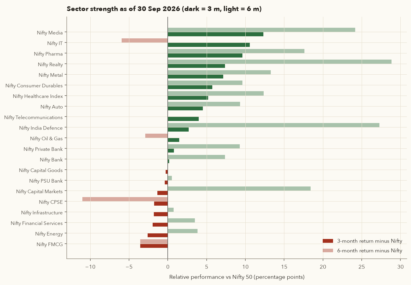
ind_close_all daily index files.How to use it: rank sectors by 3-month RS every weekend. Prefer longs in the top third and avoid the bottom third. Where 3-month and 6-month RS disagree (IT here), the shorter number is often a bounce and the longer one is the trend. Your universe may not map neatly to NSE sectors (our 37 stocks include just one pharma name), so also look at the stocks themselves (next gate).
(1) Chasing last month's top sector after it has already run 25% (look at RS and the chart). (2) Using a 1-month window alone, which is mostly noise. (3) Forgetting that in a risk-off market, "strongest sector" may just mean "falling slowest".
6. Gate 3: stock selection (liquidity and relative strength)
6.1 Liquidity filter
You must be able to get in and, more importantly, out at a fair price. Varsity suggests a tight bid-ask spread or a minimum daily volume (about 5 lakh shares). A cleaner test is turnover, because 5 lakh shares of a Rs 150 stock and of a Rs 12,000 stock are very different amounts of money.
- \(C_{t-k}\)
- The stock's close \(k\) sessions ago, in Rs (\(k = 0\) is today).
- \(V_{t-k}\)
- The number of shares traded that day.
- \(C \times V\)
- That day's turnover in Rs: roughly the money that changed hands.
- \(\operatorname{median}_{k=0..19}\)
- The middle value of the 20 daily turnovers (today and the 19 sessions before). With 20 values, it is the average of the 10th and 11th once sorted.
- \(\text{Turnover}_{20}\)
- The typical daily turnover over the last 20 sessions, in Rs (1 crore = Rs 1,00,00,000).
How it works: multiply close by volume for each of the last 20 sessions, sort the 20 numbers and take the middle one. The median is used instead of the average so that one unusually heavy day can't make a thinly traded stock look liquid. The stock passes if the result is at least Rs 20 crore.
Example (HDFCBANK, 30 Sep 2026): close 708.70 × 3,93,65,496 shares = Rs 2,789.8 crore that day. Over the 20 sessions from 2 Sep to 30 Sep the daily figure ranged from Rs 865 crore to Rs 3,611 crore. The 10th and 11th sorted values were Rs 1,982.5 crore and Rs 2,155.7 crore, so the median is about Rs 2,069 crore, far above Rs 20 crore.
On 30 Sep 2026 all 37 stocks passed. The most liquid was HDFCBANK at about Rs 2,069 crore a day. The least liquid was IRCTC at about Rs 28 crore. For a Rs 5 lakh account, liquidity is never the constraint in these names. It starts to matter with mid- and small-caps, where a Rs 1 lakh order can move the price.
6.2 Relative strength (RS) of the stock
We want the stocks that are stronger than the market: they fall less in declines and rise more in rallies. We score each stock on its 3-month (63 sessions) and 6-month (126 sessions) return minus Nifty's over the same window, then average the two.
- \(R^{(63)}_{\text{stock}}\)
- The stock's return over the last 63 sessions (about 3 months), in %. Same recipe as \(R^{(n)}\) in Section 5: today's close ÷ the close 63 sessions ago, minus 1, times 100.
- \(R^{(126)}_{\text{stock}}\)
- The stock's return over the last 126 sessions (about 6 months), in %.
- \(R^{(63)}_{\text{Nifty}},\ R^{(126)}_{\text{Nifty}}\)
- Nifty 50's return over the same two windows.
- \(\tfrac12\)
- Each horizon gets half the weight.
- \(\text{RS score}\)
- The average of the 3-month and 6-month outperformance, in percentage points.
How it works: subtract Nifty's 3-month return from the stock's, do the same for 6 months, and average the two gaps. Positive means the stock has beaten Nifty. Rank your universe by this score: the highest numbers are the leaders. The ETERNAL example below plugs in real numbers.
Computing an RS score step by step
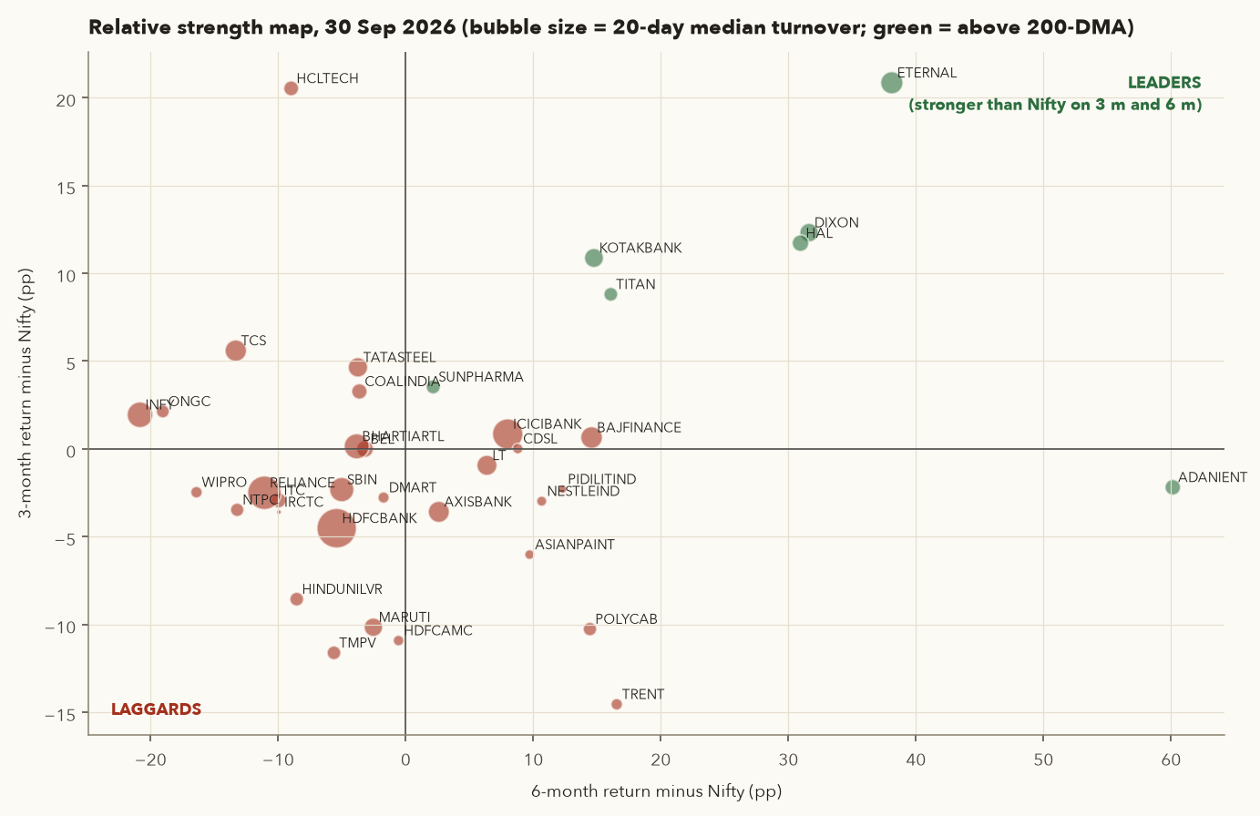
- Nifty: 63-session return −6.43%, 126-session return −0.87%.
- ETERNAL: 63-session return +14.41%, 126-session return +37.24%.
- 3-month RS = 14.41 − (−6.43) = +20.84 pp. 6-month RS = 37.24 − (−0.87) = +38.11 pp.
- RS score = ½(20.84) + ½(38.11) = +29.48, rank 1 of 37. It also closes above both its 50- and 200-DMA, one of only 3 stocks doing so.
| Rank | Stock | Close | 3m RS (pp) | 6m RS (pp) | RS score | Above 50 / 200-DMA | Turnover (Rs cr) |
|---|---|---|---|---|---|---|---|
| 1 | ETERNAL | 320.00 | +20.84 | +38.11 | +29.48 | Yes / Yes | 638 |
| 2 | ADANIENT | 2,903.40 | −2.19 | +60.14 | +28.97 | No / Yes | 313 |
| 3 | DIXON | 13,100.00 | +12.31 | +31.62 | +21.97 | No / Yes | 444 |
| 4 | HAL | 4,668.00 | +11.71 | +30.95 | +21.33 | No / Yes | 357 |
| 5 | KOTAKBANK | 417.00 | +10.87 | +14.76 | +12.81 | Yes / Yes | 465 |
| 6 | TITAN | 4,587.00 | +8.80 | +16.08 | +12.44 | No / Yes | 248 |
| … | … | ||||||
| 35 | TMPV | 283.50 | −11.62 | −5.62 | −8.62 | No / No | 244 |
| 36 | WIPRO | 158.50 | −2.47 | −16.40 | −9.44 | No / No | 173 |
| 37 | INFY | 994.10 | +1.94 | −20.83 | −9.45 | No / No | 847 |
How to use it: each weekend, rank your universe and keep a focus list of the top 10-12 names. During the week, look for setups mainly in the focus list. This mirrors Varsity's momentum-portfolio idea (rank by past return, keep the top dozen) at a swing-trading scale.
RS tells you what has been strong, not what will be. Leaders can reverse violently. Even ADANIENT's +60 pp 6-month RS sits next to a negative 3-month RS, which is a sign of fading momentum. RS is a filter to put the odds on your side, not a reason to buy on its own.
framework.indicators.relative_strength(df, bench_df, period) returns the RS line, the ratio of stock to benchmark return over period days, and Mansfield RS. The framework.scan CLI ranks candidates by a rating built from the 3- and 6-month ratios.
7. Gates 4-7: setup, trigger, stop and position size
7.1 Setup versus trigger
A setup is a chart condition that makes a move likely enough to watch, for example "price has pulled back to the 20 EMA in an uptrend". A trigger is the price event that says "the move has started, act now", for example "price trades above yesterday's high". Separating the two stops you buying falling knives: if the bounce never comes, the trigger never fires and you never enter.
7.2 The initial stop: where am I wrong?
The stop goes where your idea is proven wrong, not where the loss "feels" acceptable. Below the pullback low, below the breakout bar, below support. We add a small buffer of a fraction of ATR(14) so that ordinary noise doesn't take you out. ATR is the average true range from Chapter 4.
- \(\text{structure low}\)
- The chart price that proves the idea wrong if it breaks: the pullback low, the breakout-bar low or the pattern low. Each setup's rules say which one.
- \(b\)
- The buffer, as a fraction of ATR: 0.25 for Setups 1, 2 and 4, and 0.1 for Setup 3.
- \(\text{ATR}_{14}\)
- The 14-day average true range on the setup day, in Rs: the size of a typical day's move (Chapter 4).
- \(\text{Entry}\)
- The price you buy at, in Rs.
- \(R\)
- The risk per share, in Rs: what you lose on each share if the stop is hit exactly.
How it works: find the structure low, then subtract a small slice of ATR so that ordinary noise doesn't reach the stop. The gap between entry and stop is \(R\), your unit of risk.
Example (TITAN, Section 9): lowest low of the last 3 sessions 3,667.3, ATR 63.39, \(b = 0.25\). Stop = 3,667.3 − 0.25 × 63.39 = 3,667.3 − 15.85 = 3,651.45. Entry 3,762.00, so \(R = 3{,}762.00 - 3{,}651.45 = 110.55\) rupees per share.
\(R\) is the unit everything else is measured in. A trade that makes \(2\times\) the per-share risk is a +2R trade. A full stop-out is −1R. Thinking in R lets you compare a Rs 300 stock with a Rs 14,000 stock.
- \(\text{Entry},\ \text{Stop}\)
- Your buy price and initial stop, in Rs. \(\text{Entry} - \text{Stop}\) is \(R\), the risk per share.
- \(i\)
- Numbers each part of the exit. A trade sold in two halves has parts \(i = 1, 2\). A trade sold all at once has only \(i = 1\).
- \(\text{Exit}_i\)
- The price at which part \(i\) was sold.
- \(w_i\)
- The fraction of the position sold in part \(i\) (0.5 for a half). The fractions add up to 1.
- \(\textstyle\sum_i\)
- "Add up" over all the parts.
- \(\text{costs}\)
- Round-trip trading costs per share, in Rs. The backtests use a flat 0.24% of the entry price.
- For each part of the exit, take its profit per share (\(\text{Exit}_i - \text{Entry}\)) and multiply by its fraction \(w_i\). Add the parts. That is the average profit per share.
- Divide by \(R\) to express it in R. +2R means you made twice what you risked. −1R is a clean stop-out.
- Subtract the costs, also divided by \(R\). The tighter the stop, the bigger this deduction.
Example (TITAN, Section 9): half sold at 3,983.09 and half at 4,075.50, entry 3,762.00, \(R = 110.55\). Gross = 0.5 × 221.09/110.55 + 0.5 × 313.50/110.55 = 1.00 + 1.42 = 2.42R. Costs = 0.0024 × 3,762/110.55 ≈ 0.08R. Net = +2.34R.
7.3 Position size: the most important calculation in this course
Varsity's Module 9 opens its position-sizing chapters with a poker story: the author lost his buy-in three times in 25 minutes by betting too big after losses. The lesson is that position sizing, not stock picking, decides whether you survive. Losses compound against you:
| Account drawdown | 5% | 10% | 20% | 30% | 40% | 50% | 60% |
|---|---|---|---|---|---|---|---|
| Gain needed to get back to the start | 5.3% | 11.1% | 25.0% | 42.9% | 66.7% | 100% | 150% |
The fix is fixed-fractional risk: decide how much of the account you will lose if the stop is hit (we use 1%), then let the stop distance set the number of shares. Varsity calls this family "percentage risk" or "percentage volatility" sizing, following Van Tharp.
- \(\text{Capital}\)
- Your account size in Rs (which figure to use is Section 7.4).
- \(\text{risk\%}\)
- The share of capital you accept losing if the stop is hit: 1% in this course, less in weaker regimes (Section 4.4).
- \(\text{Entry} - \text{Stop}\)
- The risk per share, \(R\), in Rs.
- \(\lfloor x \rfloor\)
- "Floor": round down to a whole number of shares. Rounding down keeps the risk at or under budget.
- \(Q_{\text{risk}}\)
- The number of shares the risk budget allows.
- \(Q_{\text{cap}}\)
- The number of shares the 25% exposure cap allows.
- \(\min(\dots)\)
- The smaller of the two.
- \(Q\)
- The number of shares you actually buy.
- Risk budget in Rs = capital × risk%.
- Divide the budget by the risk per share and round down. That is \(Q_{\text{risk}}\).
- Divide 25% of capital by the entry price and round down. That is \(Q_{\text{cap}}\).
- Buy the smaller of the two. If the cap is smaller, your actual risk ends up below 1%, which is fine. The TITAN example below works through it.
The second term is an exposure cap: no single stock may be more than 25% of the account. Without it, a very tight stop would tell you to put the whole account in one stock, and one overnight gap would then cost far more than 1%.
Sizing the TITAN pullback trade
- Risk budget = 5,00,000 × 1% = Rs 5,000.
- Entry (buy-stop at the setup bar's high) = 3,762.00. Stop = 3,651.45. Per-share risk \(R = 110.55\).
- \(Q_{\text{risk}} = \lfloor 5{,}000/110.55 \rfloor = 45\) shares (value Rs 1,69,290, which is 34% of the account).
- \(Q_{\text{cap}} = \lfloor 1{,}25{,}000/3{,}762 \rfloor = 33\) shares.
- \(Q = \min(45, 33) = \mathbf{33}\) shares, worth Rs 1,24,146. Actual risk = 33 × 110.55 ≈ Rs 3,648 (0.73% of the account). The cap made this trade a little smaller than 1% risk, which is fine.
7.4 Which "capital"? Varsity's three equity models
When positions are already open, what number do you multiply by 1%? Varsity's Module 9 (after Van Tharp) lists three models:
- Core equity: starting capital minus money already committed to open trades. Conservative and simple.
- Total equity: cash plus the value of open positions including unrealised P&L. Aggressive: it counts paper profits before they are banked.
- Reduced total equity: core equity plus only the profit that is locked in by a trailing stop. Varsity's author prefers this one, and so do we. It rewards you for trailing stops.
Varsity also describes sizing by a fixed number of shares or lots per lakh (simple, but ignores risk), by a percentage of margin (useful for futures), and by percentage volatility: shares = (capital × x%) ÷ ATR, so each position contributes the same daily rupee swing. For ETERNAL on 30 Sep 2026, ATR(14) was 8.15. At a 1% volatility budget that gives 5,000 ÷ 8.15 = 613 shares. Compare that with 358 shares from our stop-based method in Section 17. Both are reasonable. Pick one method and use it every time.
7.5 Portfolio heat
Each trade risks ≤1%, but trades are correlated: in a sell-off, all your longs fall together. So cap the total open risk (the sum of (entry − current stop) × qty over all positions) at about 5-6% of capital, hold at most 2 positions per sector, and count a position whose stop is at breakeven as zero heat.
framework.risk.position_size(capital, risk_pct, entry, stop, lot_size=1), framework.risk.atr_stop(...) and framework.risk.r_multiple(...) implement this section. Add the 25% exposure cap in your own wrapper, or as a max_positions setting in run_backtest.
8. Gate 8: trade management and exits
Varsity's advice is blunt: once a well-checked trade is placed, do nothing until the target or the stop is hit, except trail the stop, which is "a healthy practice". We turn that into four mechanical rules that apply to every setup (Setup 3 uses a fixed target instead of rules 1-2):
- Partial profit at +2R: sell half the position when price reaches Entry + 2R. This banks a gain that already pays for about two losers.
- Breakeven stop: after the partial, move the stop on the remaining half to the entry price. The rest of the trade is now a free ride, apart from gap risk.
- Trailing exit for the rest: for daily setups, exit at the next open after a daily close below the 20 EMA. For the weekly setup, exit after a weekly close below the 10-week EMA. Using closes instead of intraday lows avoids being shaken out by one bad hour.
- Time stop: if price has not reached +1R within 10 sessions (15 for Setups 3 and 4), exit at the close. A swing trade that goes nowhere ties up capital and attention. A maximum hold (60 sessions for daily setups, 120 for the weekly one) forces a fresh look.
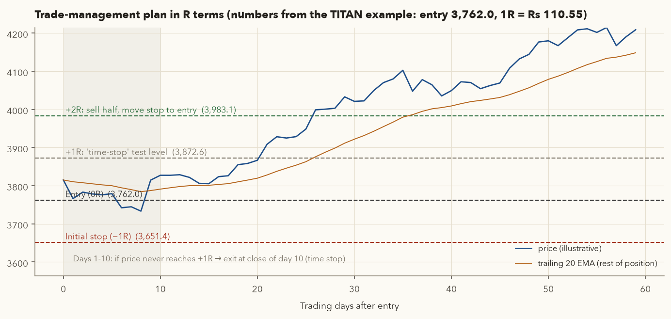
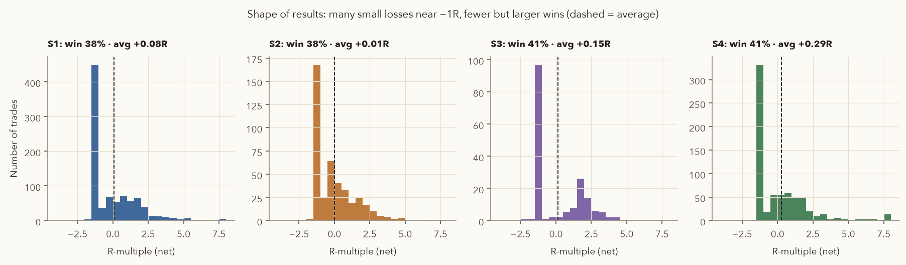
Swing-trade results are lopsided (Figure 15): most trades end near −1R or a little above zero, and a minority become large winners. The partial at 2R makes the trade less stressful to hold. The breakeven stop turns some would-be losers into scratches. The trailing stop lets the few big trends pay for everything. The time stop removes dead money. Each rule is a trade-off. A tighter trail, for example, gives back less but cuts big winners short.
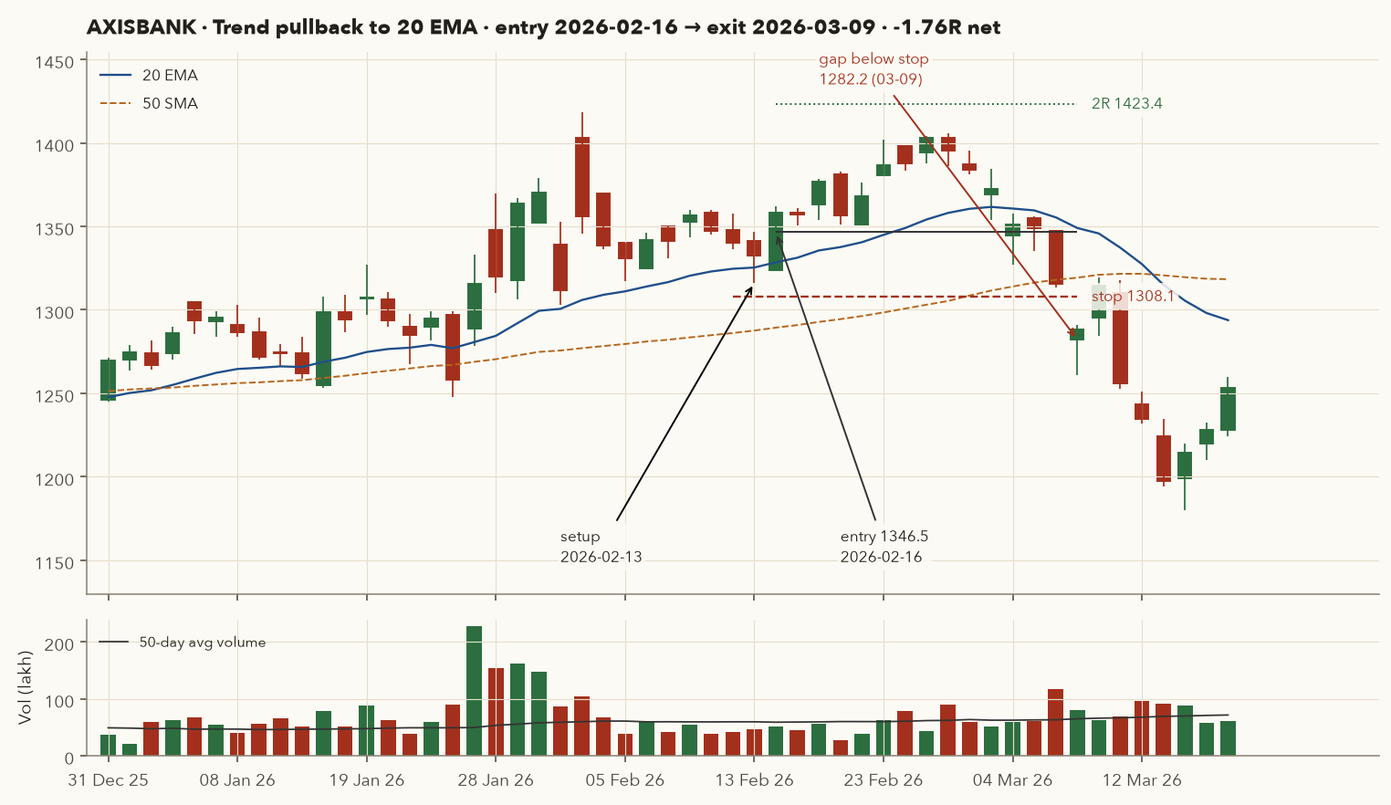
An overnight gap. If a stock closes at 1,315 and opens at 1,282 below your stop of 1,308, you sell near 1,282, not 1,308. Section 14 measures how often that happens.
9. Setup 1: trend pullback to the 20 EMA
The idea: in an established uptrend, buy a temporary dip to a rising short-term average rather than chasing strength. You get a better price and a nearby, logical stop.
The logic: trends move in waves. After a push higher, early buyers take profits and price drifts back toward its "fair" short-term level, the 20 EMA. Buyers who missed the first leg wait there. If the trend is healthy, they step in and price turns back up. If the dip goes much deeper (below the pullback low), the trend may be ending, and we want out.
Exact rules (S1)
| Step | Rule |
|---|---|
| Trend filter | Close > 50-SMA > 200-SMA; the 200-SMA is higher than 20 sessions ago; the 20 EMA is above the 50-SMA |
| Recent strength | The highest high of the last ~60 sessions was made within the last 10 sessions (a fresh high, then a dip) |
| Setup bar | Today's low ≤ 20 EMA × 1.005 (touched or came within 0.5%), and the close stays above the 50-SMA |
| Trigger | Buy-stop at the setup bar's high, valid for 3 sessions (cancel if the stop is hit first). On a gap above the trigger, the fill is at the open. |
| Initial stop | Lowest low of the last 3 sessions − 0.25 × ATR(14) |
| Management | Half at +2R, then breakeven stop and trail with a daily close < 20 EMA; time stop 10 sessions; max hold 60 |
A textbook pullback in a strong uptrend (+2.34R net)
- Context (3 Nov 2025): close 3,724.5 > 50-SMA 3,583.01 > 200-SMA 3,428.83. On 23 Oct 2025 TITAN had tagged 3,800, its highest price in more than a year (the all-time high was 3,886.95 in January 2024), so the stock had just made a fresh 52-week high. Nifty was above its 200-DMA (risk-on).
- Setup bar (3 Nov): low 3,667.3 ≤ 20 EMA 3,660.53 × 1.005 = 3,678.83. The dip touched the average. High 3,762.0 becomes the trigger.
- Stop: lowest low of 30 Oct-3 Nov = 3,667.3, minus 0.25 × ATR 63.39 (15.85) = 3,651.45. \(R = 3{,}762.00 - 3{,}651.45 = 110.55\). 2R target = 3,762 + 2 × 110.55 = 3,983.10.
- Entry (4 Nov): opened 3,724.5, rose to 3,827 and filled the buy-stop at 3,762.00. Volume that day was 25.2 lakh, about 2.4× the 50-day average, which confirmed the turn. Size: 33 shares (Section 7.3).
- Weeks 1-7: price held above the stop and climbed slowly. It never needed the time stop (it passed +1R within 10 sessions).
- Partial (26 Dec 2025): high 4,006.9 ≥ 3,983.10, so sell 16 shares at 3,983.09 (+2R). The stop on the other 17 moves to 3,762.
- Trail exit: on 20 Jan 2026 the close (4,075.5) fell below the 20 EMA (4,102.17), so sell the remaining 17 at the next open, 21 Jan, at 4,075.50.
- Result: \(R = 0.5\times\frac{3983.09-3762}{110.55} + 0.5\times\frac{4075.5-3762}{110.55} = 0.5(2.00)+0.5(2.84) = 2.42R\) gross. The backtest deducts a flat 0.24% of the entry value, 0.0024 × 3,762 / 110.55 ≈ 0.08R, giving net +2.34R. In rupees, with the real 16/17-share split and the exact costs (STT 257.16 + exchange 7.89 + SEBI 0.26 + GST 1.47 + stamp 18.62 + DP 2 × 15.34 = Rs 316.08), the trade made Rs 8,550.86 (+1.71% of the account) over 53 sessions. All R figures in this chapter use the same backtest convention (equal halves, flat 0.24% cost), so they can differ slightly from rupee P&L ÷ rupee risk.
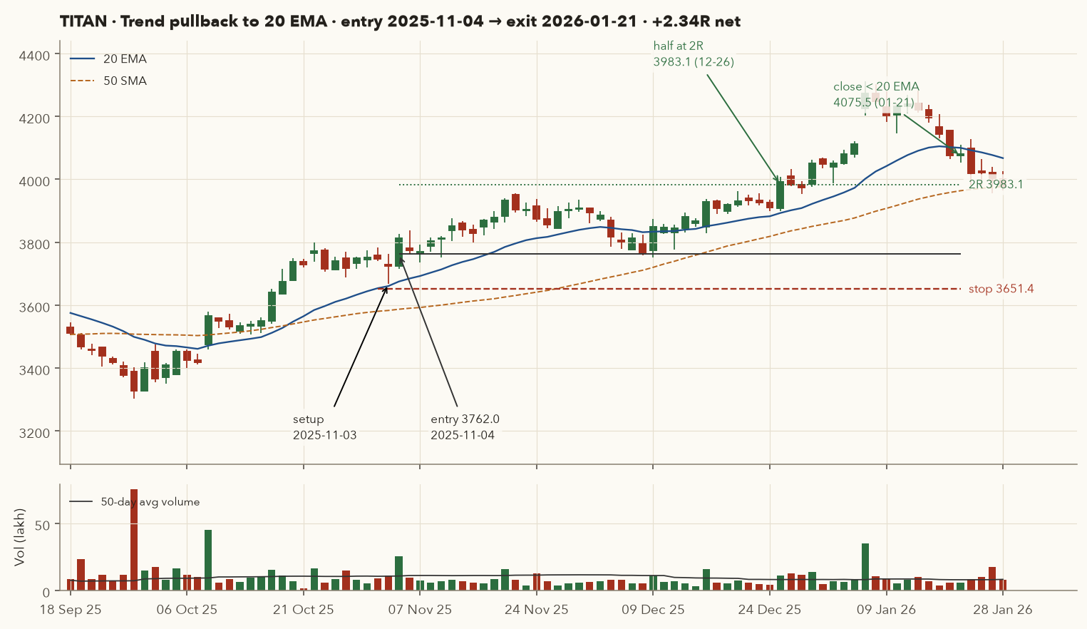
| Date | Open | High | Low | Close | 20 EMA | Close in R | Action |
|---|---|---|---|---|---|---|---|
| 31 Oct 2025 | 3,758.9 | 3,783.0 | 3,739.5 | 3,746.7 | 3,653.80 | — | Drifting back toward the EMA |
| 3 Nov 2025 | 3,730.0 | 3,762.0 | 3,667.3 | 3,724.5 | 3,660.53 | — | Setup bar: low touches the EMA. Place buy-stop 3,762 |
| 4 Nov 2025 | 3,724.5 | 3,827.0 | 3,715.0 | 3,813.5 | 3,675.10 | +0.47 | Filled at 3,762.0. Place stop GTT 3,651.45 |
| 6 Nov 2025 | 3,780.0 | 3,837.7 | 3,761.6 | 3,774.4 | 3,684.55 | +0.11 | Hold |
| 11 Nov 2025 | 3,810.5 | 3,820.0 | 3,752.1 | 3,812.4 | 3,713.54 | +0.46 | Hold |
| 26 Dec 2025 | 3,908.9 | 4,006.9 | 3,900.0 | 3,992.0 | 3,892.91 | +2.08 | 2R hit: sell 16 at 3,983.09; stop to 3,762 |
| 20 Jan 2026 | 4,155.0 | 4,155.0 | 4,064.3 | 4,075.5 | 4,102.17 | +2.84 | Close below the 20 EMA: exit tomorrow |
| 21 Jan 2026 | 4,075.5 | 4,109.9 | 4,053.5 | 4,079.2 | 4,099.98 | +2.87 | Sold 17 at the open, 4,075.5 |
Right setup, wrong market: −1.76R net
- Setup bar (13 Feb 2026): close 1,332.3, 20 EMA 1,325.32, 50-SMA 1,287.58, 200-SMA 1,197.76 (strong uptrend). Low 1,316.1 ≤ 1,325.32 × 1.005 = 1,331.95. Trigger = high 1,346.5.
- Stop: lowest low of 11-13 Feb = 1,316.1 − 0.25 × 32.16 = 1,308.06. \(R = 38.44\).
- Entry (16 Feb): opened 1,324, traded up to 1,361.9 and filled at 1,346.5. Size: risk allows 130 shares, the cap allows 92, so buy 92 (Rs 1,23,878; planned risk Rs 3,536).
- Late Feb: the stock passed +1R (1,384.94) on 23 Feb and peaked at 1,405.7 on 26 Feb (+1.54R), short of the 2R level of 1,423.38, so there was no time stop and no partial. Nifty slipped below its 200-DMA on 27 Feb 2026, and the March sell-off began (VIX rose from ~13 to above 20).
- 6 Mar: close 1,315.8, just 7.7 points above the stop (low 1,313.5).
- 9 Mar: opened at 1,282.2, below the stop of 1,308.06. The stop order fills near the open, not at 1,308.
- Result: \((1282.2 - 1346.5)/38.44 = -1.67R\) gross, −1.76R after costs. Rs −6,200 (−1.24% of the account). The loss was 1.75 times the planned risk because of the gap.
The everyday −1R
Setup bar 3 Nov 2025 (low 983.3 vs 20 EMA 990.71), entry 4 Nov at 994.55, stop 977.54 (\(R = 17.01\), only 1.71% below entry). Price slid and hit the stop on 6 Nov: −1.0R gross. 125 shares (the cap again bound) lost Rs 2,126 plus Rs 290 of costs. Note that costs were 0.14R here, because the stop was so tight. Tight stops make costs a bigger share of R. This is the most common outcome of any setup: a small, planned, boring loss.
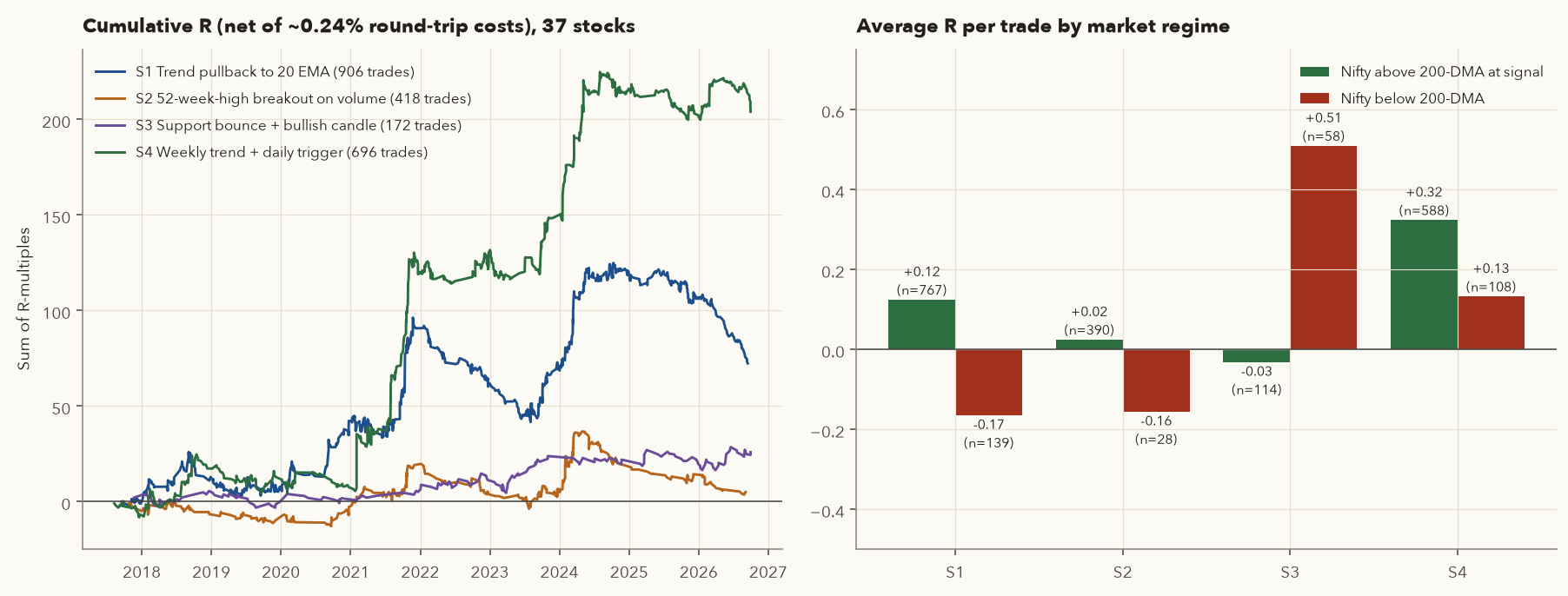
Setup 1 statistics (37 stocks, 2017-Sep 2026, net of costs): 906 trades, win rate 38.3%, average +0.080R, profit factor 1.13 (total R won ÷ total R lost; above 1 means the winners outweighed the losers), average hold 13.8 sessions. With Nifty above its 200-DMA: +0.124R (767 trades). Below: −0.166R (139 trades). In 2025-26 alone: 121 trades, win rate 24.0%, −0.399R. A choppy market is the pullback trader's worst enemy, because every "dip to the EMA" keeps going.
(1) Buying the touch without waiting for the trigger. (2) Calling a stock an "uptrend" because of one week of gains. Use the 50/200 filter. (3) Moving the stop lower "to give it room" after entry. (4) Taking pullbacks while breadth is collapsing.
framework.strategies.trend_pullback(df) returns entry, exit and stop columns for exactly this rule set. Run python -m framework.backtest_cli trend_pullback to reproduce the statistics.
10. Setup 2: breakout to a 52-week high on volume
The idea: when a stock closes above the highest price of the past year, on heavy volume, after a period of sideways movement (a "base"), buy the next morning.
The logic: the 52-week high is a resistance level everyone can see (Chapter 3). Sellers who bought near it have been waiting to "get out at cost". A close above it on unusual volume means demand has absorbed all of that supply. With nobody left holding at a loss above, there is little overhead resistance. Volume, as Varsity's volume chapter stresses, is the confirmation that big participants are involved.
Exact rules (S2)
| Step | Rule |
|---|---|
| Signal bar | Close > prior 252-session high (52-week high); volume ≥ 1.5 × prior 50-day average; close in the upper half of the day's range |
| Base | The prior 20 sessions' range (high − low) ≤ 15% of the high, i.e. a consolidation, not a vertical spike |
| Entry | Next session's open. Skip if it gaps more than 3% above the signal close (don't chase). |
| Initial stop | Lower of (signal-bar low, old 52-week high) − 0.25 × ATR(14). A close back inside the base means the breakout failed. |
| Management | Half at +2R, breakeven, trail with a close < 20 EMA; time stop 10 sessions; max 60 |
- \(V_t\)
- Volume (shares traded) on the signal day \(t\).
- \(V_{t-k}\)
- Volume \(k\) sessions before the signal day.
- \(\frac{1}{50}\sum_{k=1}^{50} V_{t-k}\)
- The average volume of the 50 sessions before the signal day. \(k\) starts at 1, so the signal day itself is left out.
- \(\text{RVOL}_t\)
- Relative volume: the signal day's volume as a multiple of that average. 1.0 = normal, 2.0 = double.
How it works: average the volume of the previous 50 sessions and divide the signal day's volume by it. The breakout counts only if RVOL is at least 1.5. The signal day is left out of the average so that a huge day can't inflate its own yardstick. The MARUTI example below has an RVOL of 7.15.
A news-driven breakout that kept going (+2.71R net)
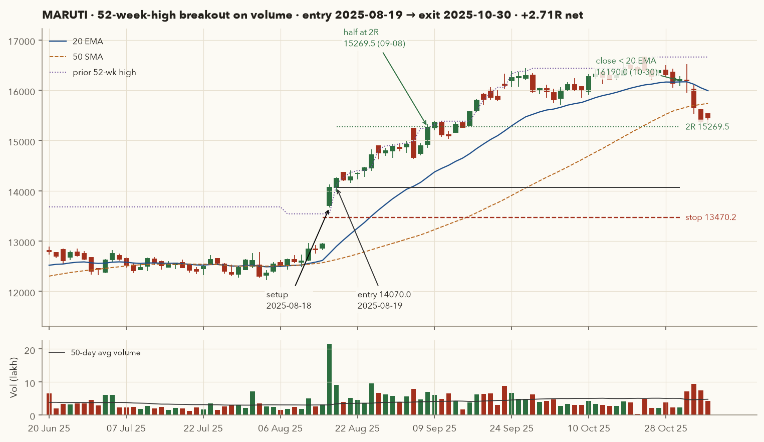
- Base: from 20 June to 14 August 2025 MARUTI moved sideways between 12,225 and 12,959 below its 52-week high of 13,541.65 (Figure 8).
- Signal (18 Aug 2025): close 14,068 > 13,541.65. Volume 21,54,781 vs a 50-day average of 3,01,425, so RVOL = 7.15. The close was near the day's high. (The surge followed the government's mid-August 2025 signal of GST rate cuts, which lifted auto stocks. The chart rules didn't need to know that.)
- Entry (19 Aug): open 14,070 (a 0.01% gap, within the 3% limit).
- Stop: min(signal low 13,664, old high 13,541.65) − 0.25 × 285.59 = 13,470.25. \(R = 599.75\) (4.26%).
- Size: \(\lfloor 5000/599.75\rfloor = 8\) shares (the cap also allows 8). Value Rs 1,12,560. Planned risk Rs 4,798.
- Partial (8 Sep): high 15,319 ≥ 2R level 15,269.49. Sell 4 shares. Stop on the other 4 moves to 14,070.
- Exit: 29 Oct close 16,138 < 20 EMA 16,160.25, so sell 4 at the 30 Oct open, 16,190.
- Result: \(0.5(2.00) + 0.5\frac{16190-14070}{599.75} = 1.00 + 1.77 = 2.77R\) gross, +2.71R net, Rs +12,983 (+2.60%) in 49 sessions.
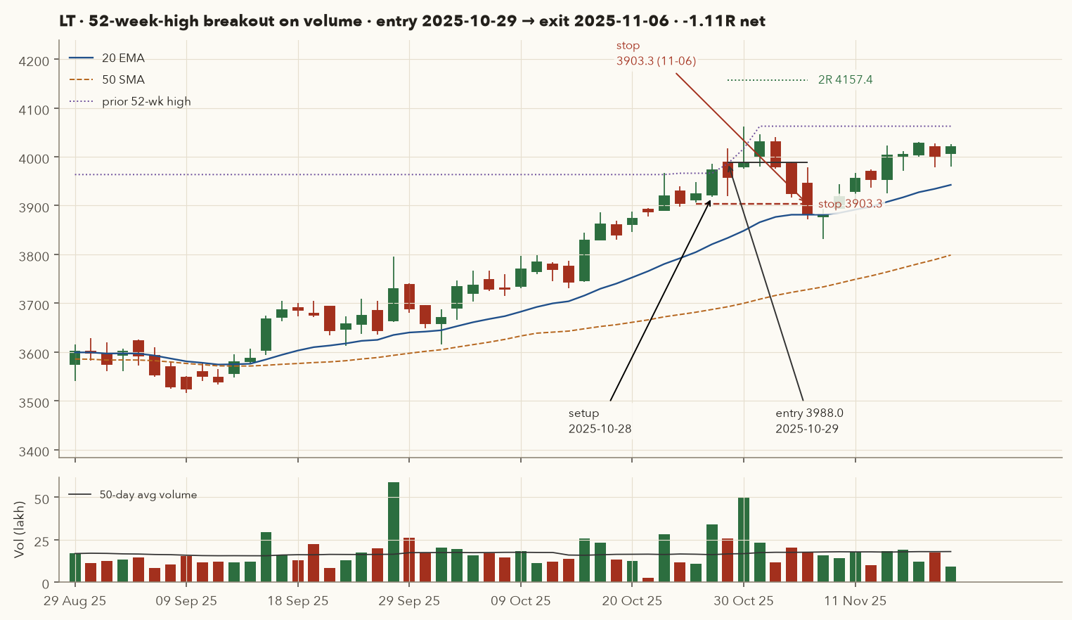
A breakout that just didn't follow through (−1.11R net)
- Signal (28 Oct 2025): close 3,972.8 > prior 52-week high 3,966.2, by only 0.17%. RVOL = 33.9 lakh / 16.1 lakh = 2.11. RSI(14) 75: already stretched.
- Entry (29 Oct): open 3,988.0. Stop = 3,917.3 − 0.25 × 55.93 = 3,903.32. \(R = 84.68\). Size 31 shares (the cap binds).
- Price poked to 4,062.6 on 30 Oct (still under +1R = 4,072.7), then faded.
- 6 Nov: low 3,872.1 < stop, so out at 3,903.32. −1.0R gross, −1.11R net (Rs −2,913).
- And then: after one more dip to 3,831.1 on 7 Nov, LT recovered and closed at 4,081.3 on 27 Nov, above the entry. Stops sometimes take you out just before a move resumes. That is the cost of having a stop at all, and re-entry only happens if a new setup appears.
- Lesson: a breakout that only just clears the level, with modest volume, is weaker evidence than MARUTI's 7× volume and a close 3.9% above the old high. Many traders require RVOL ≥ 2 and a close at least 1% above the level. You can test those refinements in Chapter 12.
A breakout entered just before the Union Budget
- Signal: ONGC broke out on 28-29 Jan 2026 on 4.7× average volume (close 275.39 on 29 Jan vs the prior 52-week high of 269.65).
- Entry (30 Jan): 273.89, stop 267.40 (\(R = 6.49\)). The 25% cap allowed 456 shares, a planned risk of about 0.6% of the account.
- The event: the Union Budget was presented on Sunday 1 Feb 2026, and NSE held a special live trading session that day (NSE circular, Jan 2026). Our Yahoo daily series doesn't contain that Sunday session. The next bar in our data is 2 Feb, opening at 251.60, far below the stop.
- Could you even have sold on Sunday? Probably not. NSE declared 1 Feb a settlement holiday, and brokers' notices said shares bought on 30 Jan would reach demat only on 2 Feb, so they could not be sold in the Budget session (no BTST, i.e. buy-today-sell-tomorrow).
- Result: the stop was jumped by an event. In our data the loss is −3.44R gross, −3.54R net, about −2.1% of the account against a planned 0.6%.
- Lesson: know the event calendar. Budget day, RBI policy days and company results are scheduled. Don't open a fresh breakout the session before one, or halve the size.
Setup 2 statistics: 418 trades, win rate 37.8%, average only +0.012R (gross +0.073R before costs), profit factor 1.02. It was positive in 2021-23 (+0.176R) and clearly negative in 2024-26 (−0.268R, win rate 29.6%). On our large-cap list, plain 52-week-high breakouts were roughly break-even after costs. That doesn't make breakouts useless. It means the edge, if any, comes from selectivity (base quality, sector strength, volume quality) and from the occasional MARUTI-style runner.
framework.strategies.breakout_52w(df), with the volume and base conditions as parameters, so you can test RVOL 1.5 vs 2.0 yourself.
11. Setup 3: support bounce with a bullish candle (the Varsity checklist)
This setup is a direct translation of the trading checklist in Varsity Module 2's finale chapter. In Varsity's words, the checklist is "fairly stringent", so few trades qualify, but conviction is high when one does. Here are its items, and how we made each one exact:
| Varsity checklist item | Our exact rule |
|---|---|
| A recognisable candlestick pattern in the last 1-3 candles | Hammer, bullish engulfing, piercing or morning star (definitions from Chapter 2) |
| Prior trend should be down for a bullish pattern | Close today < close 10 sessions ago |
| Volume at least equal to the 10-day average | Volume ≥ average of the prior 10 sessions |
| Support should coincide with the stop-loss; reject if S&R is more than 4% away from the stop | A confirmed swing low from 15-250 sessions ago within 3% of the pattern low; that support within 4% of the stop |
| Look back ~2 years for S&R | Pivot lows and highs (5 bars either side) within the last 250 sessions |
| Target from the nearest resistance; minimum RRR 1.5 | Target = nearest swing high above entry; skip unless \((T-E)/(E-S) \ge 1.5\) |
| MACD / RSI as optional confirmation | Not required (kept simple) |
| Stop = low of the pattern | Pattern low − 0.1 × ATR(14) |
Entry: buy-stop above the pattern high, valid for 2 sessions. Exit: the full position at the target or at the stop. The time stop applies if price has not reached +1R within 15 sessions, and the maximum hold is 40 sessions. There is no partial exit or trailing here, because the target is a real resistance level.
- \(\text{Target}\)
- Where you plan to take profit: the nearest swing high (resistance) above entry, in Rs.
- \(\text{Entry}\)
- The planned buy price: the buy-stop just above the pattern high.
- \(\text{Stop}\)
- The initial stop: pattern low − 0.1 × ATR(14).
- \(\text{RRR}\)
- Risk-reward ratio: rupees you stand to make for each rupee you risk.
How it works: divide the distance to the target by the distance to the stop. An RRR of 1.5 means a winner pays 1.5 times what a loser costs. Below 1.5, skip the trade. The AXISBANK example below has a planned RRR of 4.3.
The logic: support is a price where buyers showed up before. A bullish candle there, on decent volume, shows they are showing up again. The stop sits just under the pattern, so it is close and the reward to the next resistance can be several times the risk. The weakness: you are buying in a short-term downtrend, so when support breaks, it can break hard.
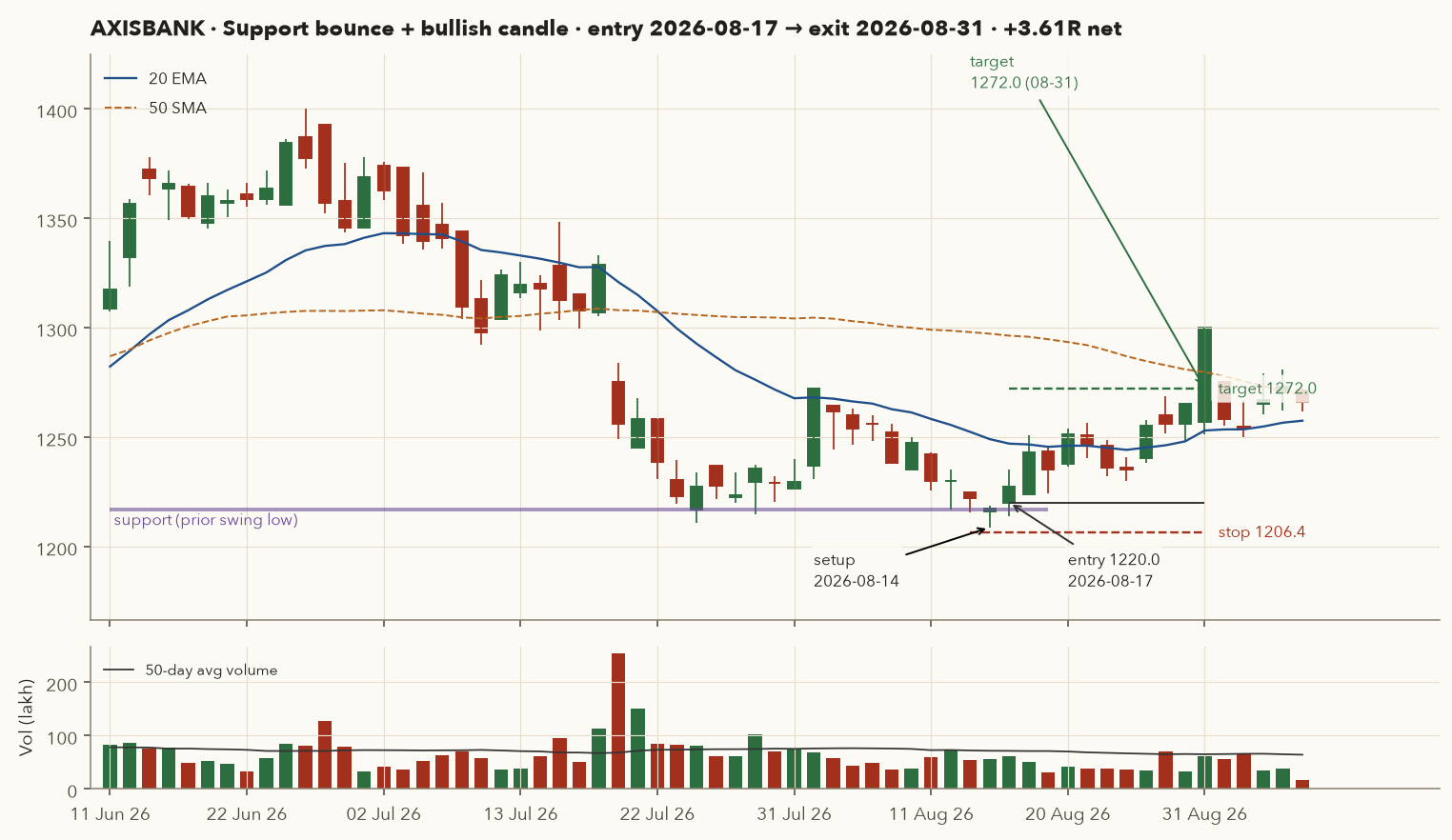
Hammer on a December swing low (+3.61R net)
- Support: the swing low of 1,216.9 made on 16 Dec 2025.
- Prior trend: AXISBANK closed between about 1,307 and 1,329 in mid-July 2026, then slid to 1,217.4 by 14 August. Close on 14 Aug (1,217.4) was below the close 10 sessions earlier. ✓
- Pattern (14 Aug 2026): O 1,216.0, H 1,218.7, L 1,208.6, C 1,217.4. Body 1.4, lower shadow 7.4 (≥ 2 × body), upper shadow 1.3 (≤ 25% of the 10.1 range). A hammer. ✓
- Volume: 55.6 lakh vs 10-day average 54.7 lakh (1.02×). ✓ Just enough.
- Stop: 1,208.6 − 0.1 × 21.87 = 1,206.41. Support 1,216.9 is 0.9% above the stop (well within 4%). ✓
- Target: nearest swing high above = 1,272.0 (3 Aug 2026). Planned RRR = (1,272.0 − 1,218.7)/(1,218.7 − 1,206.41) = 4.3 ≥ 1.5. ✓
- Entry (17 Aug): opened at 1,220.0, above the trigger 1,218.7, so filled at the open. \(R = 13.59\) (1.11%).
- Size: risk allows 367 shares (Rs 4.48 lakh, 90% of the account!). The 25% cap allows 102, so actual risk is only Rs 1,386. This shows why the cap exists.
- Exit (31 Aug): high 1,300 ≥ 1,272, so sold at the target 1,272.0. +3.83R gross, +3.61R net (Rs +5,006, +1.0%), 10 sessions. The market was in risk-off mode (Nifty below its 200-DMA), which is when this setup has historically done best.
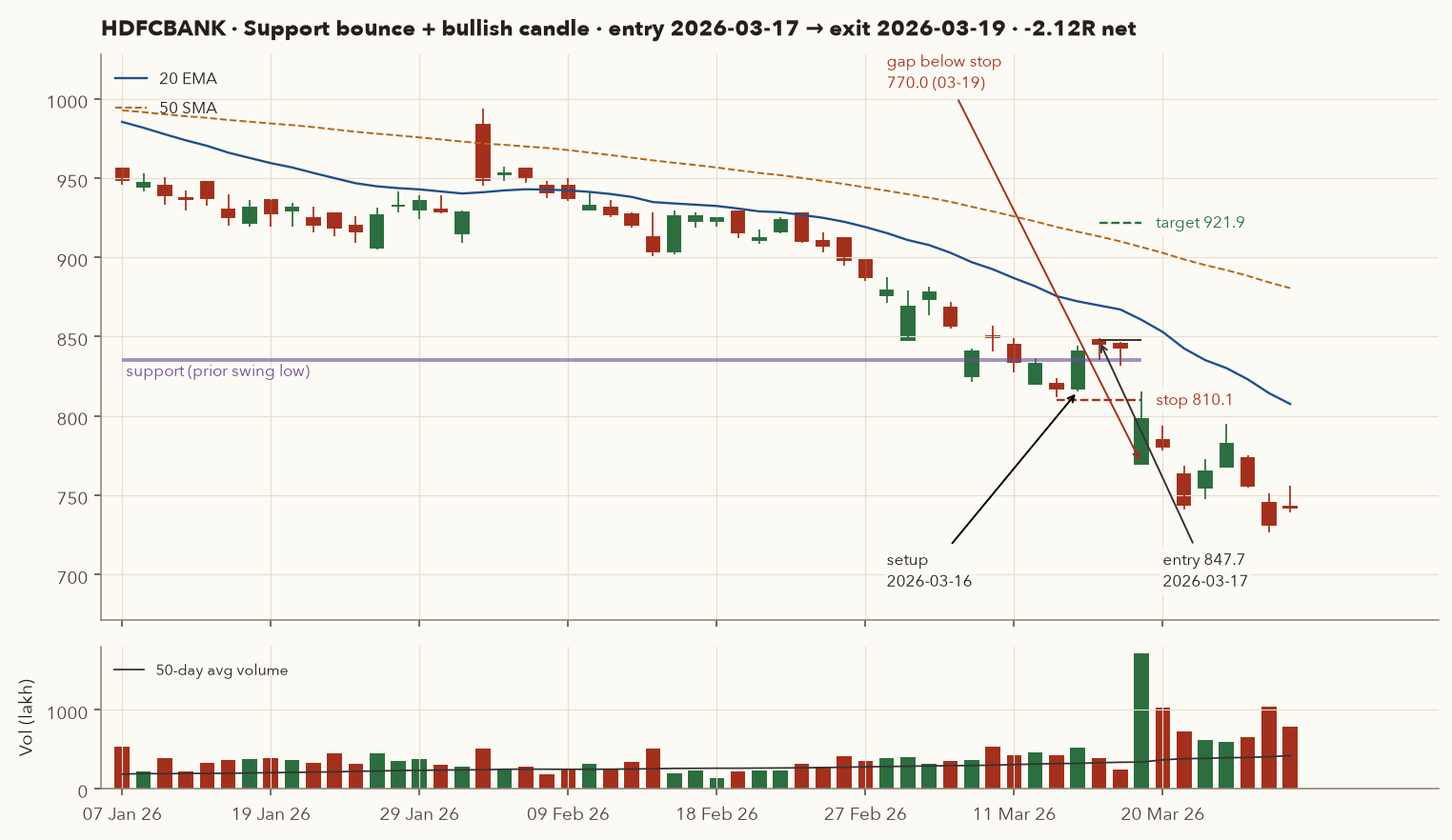
Engulfing pattern at support, then an 8.7% gap down (−2.12R net)
- Support: the swing low of 835.03 (11 Mar 2025). Price had undercut it to 812 and closed back above it.
- Pattern (16 Mar 2026): 13 Mar red (O 820.0, C 817.0), 16 Mar green (O 817.0, C 840.6), engulfing the prior body: bullish engulfing. Volume 5.22 crore vs 10-day average 3.97 crore (1.31×). RSI 34.5.
- Stop: pattern low 812.0 − 0.1 × 19.36 = 810.06. Target: swing high 921.85 (25 Mar 2025). RRR = (921.85 − 844.5)/(844.5 − 810.06) = 2.25. ✓
- Entry (17 Mar): opened 847.7, above the 844.5 trigger. \(R = 37.64\) (4.44%). Size 132 shares, risking Rs 4,968.
- 19 Mar: the stock opened at 770.0, an 8.7% gap below the previous close of 843.05 and 40 points below the stop. Volume that day was 17.2 crore, more than 5× normal.
- Result: −2.06R gross, −2.12R net, Rs −10,510 (−2.1% of the account), twice the planned loss.
- What the regime said: Nifty was below its 200-DMA, breadth was below 20% and VIX was around 19-23. The playbook allows S3 in risk-off only at half risk. At 0.5% risk this loss would have been about −1.05% of the account. The half-size rule exists for exactly this kind of day.
Hammer at the January low (+3.08R net)
Hammer on 3 Mar 2025 (O 3,425.0, H 3,472.0, L 3,340.0, C 3,453.2; lower shadow 85 vs body 28.2) at the 14 Jan 2025 swing low of 3,443.0, on volume 1.76× its 10-day average. Stop 3,329.21, target 3,920.45 (6 Dec 2024 swing high), RRR 3.14. The buy-stop at 3,472.0 filled on 5 Mar (the second valid day). The target was hit on 21 Mar: +3.14R gross, +3.08R net, Rs +15,394 on 35 shares (+3.08% of the account) in 10 sessions. This was also a risk-off market (Nifty below its 200-DMA in March 2025), just before the April-June 2025 recovery.
Setup 3 statistics: 172 trades (the checklist is strict!), win rate 40.7%, average +0.150R, profit factor 1.23, average hold 6.5 sessions. Opposite to the trend setups: with Nifty below its 200-DMA it averaged +0.509R (58 trades, 51.7% wins), and above it −0.033R (114 trades). 2025-26: 48 trades, +0.081R. Adding a "stock above its 200-SMA" filter made it worse (74 trades, +0.099R). The bounces that worked best came in washed-out markets. Treat these splits with care: 58 trades is a small sample.
12. Setup 4: weekly trend + daily trigger
The idea: use the weekly chart to decide direction (only stocks in a weekly uptrend) and the daily chart to time the entry after a short pullback. This is the multiple-timeframe approach Varsity hints at when it says higher timeframes give more reliable signals. It is also the most "positional" of the four setups.
The logic: weekly bars filter out daily noise, so a weekly uptrend reflects the bigger players' sustained buying. Inside it, short pullbacks (daily RSI dipping below 45) are pauses. A daily close above the prior two highs shows buyers are back. Because the trailing exit is weekly, the trade can last for months, which is where large R-multiples come from.
Exact rules (S4)
| Step | Rule |
|---|---|
| Weekly trend (last completed week) | Weekly close > 30-week SMA; the 30-week SMA is higher than 4 weeks ago; 10-week EMA > 30-week SMA |
| Daily pullback | RSI(14) was below 45 at some point in the last 5 sessions |
| Daily trigger | Close > the highs of both of the previous 2 sessions, and the daily close is still above the 30-week SMA |
| Entry | Next open (skip if it gaps more than 3% above the trigger close) |
| Initial stop | Lowest low of the last 10 sessions − 0.25 × ATR(14); skip if the stop is more than 10% away |
| Management | Half at +2R, breakeven, then exit the rest after a weekly close < 10-week EMA; time stop 15 sessions; max 120 |
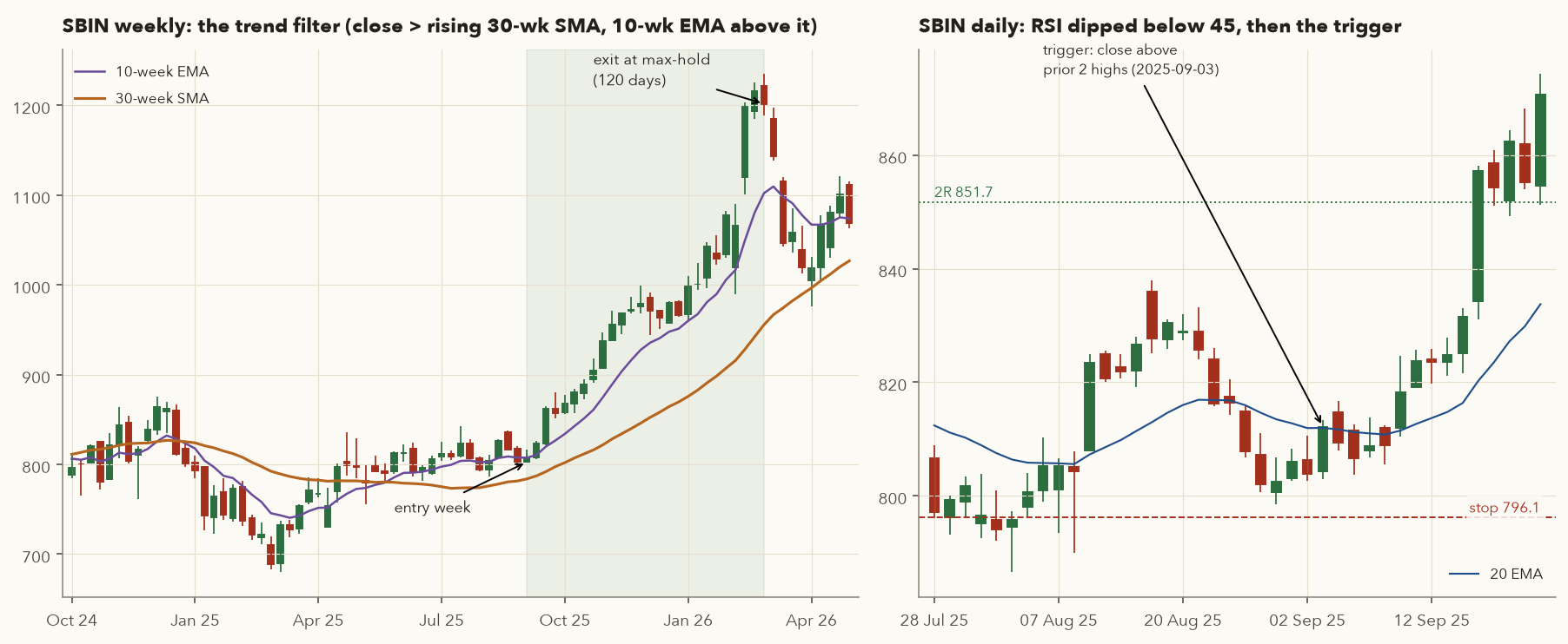
Riding the weekly trend for 120 sessions (+11.34R net)
- Weekly filter (week ending 29 Aug 2025): close above a rising 30-week SMA (781.49); 10-week EMA 807.63 above it. ✓
- Pullback: daily RSI fell to 42.7 on 2 Sep 2025. ✓
- Trigger (3 Sep): close 812.15 > highs of 1 Sep (808.3) and 2 Sep (810.5). ✓
- Entry (4 Sep): open 814.65. Stop: 10-day low 798.50 − 0.25 × 9.48 = 796.13. \(R = 18.52\) (2.27%).
- Size: risk allows 269 shares, the cap allows 153 (Rs 1,24,641; risk Rs 2,834).
- Partial (17 Sep): a 1.72 crore-share day pushed the high to 858.15 ≥ 2R level 851.69. Sell 76 shares. Stop on the other 77 moves to 814.65.
- The hold: SBIN never had a weekly close below its 10-week EMA for five months, through two quarterly results (November 2025 and February 2026).
- Exit (27 Feb 2026): 120-session maximum hold, sold at the close, 1,201.70.
- Result: \(0.5(2.00) + 0.5\frac{1201.70-814.65}{18.52} = 1.00 + 10.45 = 11.45R\) gross, +11.34R net. Rs +32,276 (+6.46% of the account) from one trade with only Rs 2,834 at risk.
Up +1.2R, then all the way back to the stop (−1.04R net)
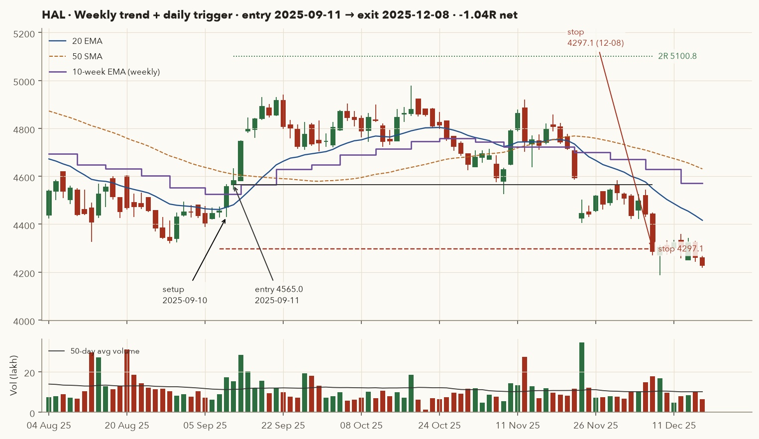
- Trigger (10 Sep 2025): close 4,557.5 above the prior two highs. Weekly trend up (10-week EMA 4,525.95 > 30-week SMA 4,376.47). Daily RSI had dipped to 40.9 on 5 Sep.
- Entry (11 Sep): 4,565.0. Stop 4,297.10 (\(R = 267.90\), 5.87%). Size 18 shares (Rs 82,170), risk Rs 4,822.
- 17 Sep: close 4,890.2 = +1.21R. Then the rally stalled well short of the 2R level (5,100.8).
- No time stop, because it had passed +1R. No partial, because it never reached +2R. So the stop stayed at 4,297.10 while the stock drifted down over October and November.
- 8 Dec 2025: low 4,270.5 hit the stop. −1.0R gross, −1.04R net (Rs −5,015) after 59 sessions.
- Lesson: wide, patient stops let winners like SBIN run, and the price is trades like this that give back an open gain. A common variant moves the stop to breakeven at +1R. That would have turned HAL into a scratch but also cut some later winners. Test variants on your data (Chapter 12) before changing rules.
A wide stop that survived March 2026 (+2.68R net)
RSI dipped to 37.5 on 29 Jan 2026. Trigger 3 Feb 2026, entry 4 Feb at 4,087.0, stop 3,820.62 (6.52% away; only 18 shares). Nifty fell about 14% from its February high close (25,953.85) to 22,331.40 on 30 Mar 2026, but TITAN held its 10-session-low stop. It reached 2R (4,619.76) on 7 Jul 2026, and the remaining 9 shares were sold at the 120-session limit on 3 Aug at 5,000.0. +2.71R gross, +2.68R net, Rs +12,804. A relative-strength leader (Figure 4) can survive a weak market. A tight stop would not have survived the March volatility.
Setup 4 statistics: 696 trades, win rate 41.4%, average +0.293R, profit factor 1.53, average hold 27.5 sessions, best trade +21.57R. It was the best of the four, and its edge came from a few long-held trends (the median trade was −0.68R). Regime: +0.323R above the 200-DMA (588 trades) vs +0.132R below (108). 2025-26: 104 trades, 30.8% wins, −0.162R.
Combine framework.data.resample(df, "W-FRI") with framework.indicators.ema/sma for the weekly filter, and framework.indicators.rsi for the daily dip. framework.strategies.ma_crossover and donchian_trend are slower cousins of this setup.
13. How the four setups did, 2017-2026 (honest numbers)
Varsity's Module 10 opens by defining a trading system: an approach you can write down as a process, with inputs, rules and outputs, that can be measured and backtested. Anything you can't define as a process isn't a system. Here we measure our four.
Method: the rules above, applied mechanically to 37 NSE stocks with daily data from Oct 2016 to 30 Sep 2026 (trades start in 2017 once the 200-day averages exist). One open trade per stock per setup. Costs of 0.24% of the entry value are deducted from every trade. When a bar touches both the stop and the target, we assume the stop was hit first. Gaps through stops fill at the open.
| Metric (net of costs) | S1 Pullback | S2 Breakout | S3 Support bounce | S4 Weekly+daily |
|---|---|---|---|---|
| Trades | 906 | 418 | 172 | 696 |
| Win rate | 38.3% | 37.8% | 40.7% | 41.4% |
| Average R (expectancy) | +0.080 | +0.012 | +0.150 | +0.293 |
| Average R before costs | +0.152 | +0.073 | +0.247 | +0.347 |
| Median R | −1.02 | −0.37 | −1.05 | −0.68 |
| Average win / average loss | +1.76 / −0.96 | +1.42 / −0.84 | +1.97 / −1.10 | +2.06 / −0.95 |
| Profit factor | 1.13 | 1.02 | 1.23 | 1.53 |
| Average hold (sessions) | 13.8 | 14.4 | 6.5 | 27.5 |
| Best / worst trade | +12.41 / −2.29 | +6.53 / −3.54 | +4.05 / −2.12 | +21.57 / −2.14 |
| Median stop distance | 3.5% | 4.6% | 2.76% | 5.16% |
| Median cost per trade (in R) | 0.069 | 0.052 | 0.087 | 0.047 |
| Longest losing streak | 16 | 12 | 6 | 16 |
| Nifty > 200-DMA: trades / avg R | 767 / +0.124 | 390 / +0.024 | 114 / −0.033 | 588 / +0.323 |
| Nifty < 200-DMA: trades / avg R | 139 / −0.166 | 28 / −0.157 | 58 / +0.509 | 108 / +0.132 |
| 2017-2020 avg R (n) | +0.19 (273) | +0.01 (128) | +0.03 (50) | +0.26 (208) |
| 2021-2023 avg R (n) | +0.15 (360) | +0.18 (182) | +0.38 (58) | +0.60 (285) |
| 2024-Sep 2026 avg R (n) | −0.12 (273) | −0.27 (108) | +0.03 (64) | −0.11 (203) |
| 2025-26 only: trades / win / avg R | 121 / 24.0% / −0.399 | 39 / 28.2% / −0.329 | 48 / 39.6% / +0.081 | 104 / 30.8% / −0.162 |
Reading the numbers: expectancy
- \(E[R]\)
- Expectancy: the average R you can expect per trade over many trades.
- \(p_{\text{win}}\)
- The win rate as a fraction: the share of trades that ended with a profit (0.414 = 41.4%).
- \(1-p_{\text{win}}\)
- The share of trades that lost.
- \(\overline{R}_{\text{win}}\)
- The average R of the winning trades (a positive number). The bar on top means "average".
- \(\overline{R}_{\text{loss}}\)
- The average R of the losing trades, kept as a negative number (for example −0.95).
How it works: weight the average win by how often you win, weight the average loss by how often you lose, and add the two. Above zero means the setup made money per trade on average (after costs, since these R values are net). Multiply by your rupee risk per trade to get rupees per trade. The S4 numbers below show the arithmetic.
For S4: \(0.414 \times 2.06 + 0.586 \times (-0.95) = 0.85 - 0.56 = +0.29R\) per trade. Risking Rs 5,000 per trade (full 1%), that's about Rs 1,465 per trade on average, before tax, across hundreds of trades. Any single month can be far worse. S1 and S4 both had 16 losses in a row at some point. Varsity calls the belief that "after 6 losses the 7th must win" the gambler's fallacy: each trade has the same odds as the first. The antidote is fixed position sizing, not bigger bets after losses.
Caveats: why these numbers are probably too good
- Survivorship bias. Our 37 stocks are today's large, successful names. Stocks that collapsed and left the index over 2016-2026 aren't in the list. Long-only trend setups on today's winners look better than they would have looked in real time.
- Correlated trades. The 2,192 trades are not independent. Many happen in the same weeks, so the true range of outcomes is wider than the trade count suggests.
- Fills. We assumed fills exactly at trigger prices (except gaps). Real GTT limit orders may fill a little worse or not at all. Costs are included, but taxes and slippage beyond 0.24% are not.
- Data quirks. Yahoo daily data. We back-adjusted the Tata Motors demerger (Oct 2025), a Trent price rescale (Jan 2026) and early CDSL data. The 1 Feb 2026 Budget Sunday session is missing. Zero-volume holiday rows were dropped.
- Regime dependence. 2021-23 was excellent and 2024-26 poor. A system that "worked" over ten years can lose for two straight years. That is normal, and it's the hardest part to live through.
- Not optimised (good), but sensitive to choices. Parameters were set before testing. As a robustness check, forcing every stop to be at least 1 × ATR away barely changed anything: S1 +0.073R, S2 +0.004R, S3 +0.099R, S4 +0.295R. That suggests the results don't hinge on one lucky parameter.
None of these setups is a money machine. On large caps, after costs, S1 and S2 have a thin edge that disappears in bad regimes. S3 is rare and has a small sample. S4 had the best long-run expectancy, but it too lost in 2025-26. Your edge comes from the whole playbook combined: regime filter, leaders only, strict sizing, event awareness and discipline. No single pattern provides it. Paper-trade or trade very small for at least 30-50 trades before trusting any setup with real size.
14. Event risk: results days, gaps and the Budget
Swing trades are held overnight, so they are exposed to news that arrives when the market is closed. The biggest scheduled source is quarterly results. Under SEBI's LODR Regulations, listed companies must publish quarterly results within 45 days of the quarter end (60 days for the annual results) and must announce the board-meeting date in advance. That gives you a calendar to plan around.
How much more do stocks move around results?
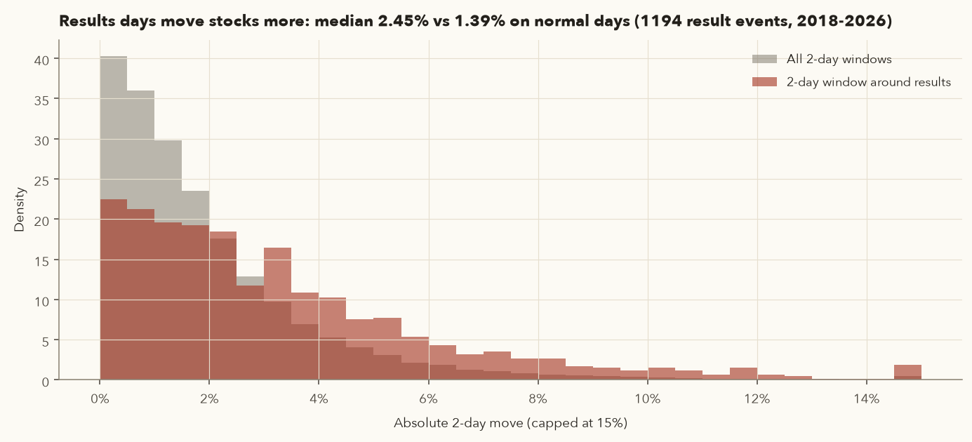
- For each results date (from Yahoo Finance's earnings calendar), measure the move from the close before the announcement to the close of the first session after it (a 2-day window), and the largest opening gap in that window.
- Median 2-day move: 2.45% around results vs 1.39% for any 2-day window.
- Moves bigger than 5%: 21.1% of results events vs 7.0% of normal windows, three times as often.
- Opening gaps bigger than 3%: 17.8% of results windows (the larger of the two opening gaps) vs 3.4% of ordinary two-session windows (1.8% of single days): about five times as often on a like-for-like basis.
- Biggest 2025-26 results moves in our list: ETERNAL (21 Jul 2025) 16.6% with a 7.8% gap; ETERNAL (20 Jan 2025) 13.8%; DIXON (20 Jan 2025) 12.1%; ADANIENT (3 Feb 2026) 11.7% with a 7.7% gap; SBIN (8 May 2026) 10.8%; CDSL (25 Jan 2025) 10.4%.
Rules for results and other events
- Know the date before you enter. Check the company's board-meeting announcement on the NSE corporate filings page. Your broker app also shows upcoming results.
- Don't open a new swing trade within ~5 sessions of results unless you accept a possible 2R-3R loss. Or enter at half size.
- Already in a trade? If it's at +2R with half booked and the stop at breakeven, holding through results is reasonable: the worst realistic case is a small loss on the remaining half. If it's still near entry, many traders exit before results, or cut to half.
- Market-wide events: the Union Budget, RBI policy, election results and global shocks can all gap every stock at once. ONGC (Section 10) is our example.
In our backtest, S1 trades that were open over a results date averaged +1.25R (201 trades), versus −0.25R for the rest. S4 showed the same pattern: +1.55R vs −0.42R. Does holding through results make money? No. Losing trades get stopped out within days, so they rarely live long enough to reach a results date. Only trades that were already working survive that long. Results days didn't cause the gains. Survival caused the overlap. Always ask "could the selection itself explain this number?" before acting on a statistic.
Upcoming results in our universe (estimated dates from Yahoo Finance; confirm on NSE): TCS ~8 Oct 2026, DMART ~10 Oct, HCLTECH ~12 Oct, ETERNAL / WIPRO / POLYCAB / NESTLEIND / HDFCAMC ~15 Oct, RELIANCE / DIXON ~16 Oct, the large private banks ~17 Oct, INFY ~23 Oct, and LT, ITC, MARUTI, ASIANPAINT, COALINDIA and others in late October. Any trade opened in early October 2026 is very likely to run into results.
15. Placing the orders: GTT mechanics
A normal stop-loss order on an Indian exchange is a day order: it expires at the close. For multi-day trades you would have to re-enter it every morning. Brokers solve this with GTT (Good Till Triggered) orders. Per Zerodha's GTT support documentation (accessed Oct 2026):
- A GTT is a trigger stored by the broker, not at the exchange. When the last traded price crosses your trigger during market hours, the broker sends an order to the exchange: either a limit order at your chosen limit price, or a market order with market protection (a market order that won't fill beyond a set band from the last price). For stocks in the F&O segment, GTTs on the stock trigger only until 3:15 pm.
- Single GTT: one trigger (buy or sell). OCO (one-cancels-other) sell GTT: a stop trigger and a target trigger on holdings. When one fires, the other is cancelled. Kite also offers an optional trailing stop-loss on GTTs (the stop trigger moves up by a fixed number of points as price rises). Our trailing rule is based on daily closes versus the 20 EMA, so we trail by hand instead.
- Valid for up to 365 days or until triggered. A GTT fires even if the stock opens beyond the trigger on a gap. A trigger fires only once: if the resulting order doesn't fill by the close, it is cancelled like any day order and you must place a fresh one.
- No funds are blocked when you create a GTT. Margin and funds are checked at trigger time. Sell GTTs on your holdings must be authorised with your CDSL TPIN (a PIN from the depository that approves shares leaving your demat account).
- GTTs are cancelled when the stock has a corporate action (bonus, split, rights issue, amalgamation) whose impact is more than 2% of the market value on the ex-date or record date. Re-place them afterwards.
- Placing a GTT is free, and Zerodha allows up to 500 active GTTs per account. Other brokers have similar orders under different names. Check yours.
The order sequence for one swing trade
- Evening of 3 Nov (setup found): create a single buy GTT for 33 shares, trigger 3,762.00, limit about 0.3-0.5% higher (e.g. 3,775) so the order can fill if price moves fast. Note the limit means you might pay a little more than our backtest assumed.
- Evening of 4 Nov (filled at ~3,762): create the exit orders. With a half-at-2R plan, either (a) an OCO sell GTT for 16 shares with stop trigger 3,651.45 (limit a little lower, e.g. 3,640) and target trigger 3,983.10, plus a single sell GTT stop for the other 17 shares at 3,651.45, or (b) one stop GTT for all 33 and a separate target GTT for 16. Check how your broker treats quantities across multiple GTTs on the same holding.
- Each evening: 2 minutes. Is the position above the stop? Has the 20 EMA been broken on a close? Any results date coming?
- 26 Dec (2R hit, 16 sold): modify the remaining stop GTT up to 3,762.00 (breakeven).
- 20 Jan (close below the 20 EMA): place a sell order for the 17 shares for the next morning (an AMO, i.e. an after-market order placed in the evening for the next open, at market or with a limit near the expected open), and cancel the stop GTT once it fills.
If a stock gaps below your stop and below your limit price, as on AXISBANK 9 Mar 2026 or HDFCBANK 19 Mar 2026, the GTT fires but its limit sell may not fill, and the stock keeps falling. On a gap day, check your positions after the open and exit manually if your limit is stranded. Two ways to reduce this risk: set the stop's limit price a few percent below the trigger, or choose the GTT's market-with-protection option for stop exits. Both raise the chance of a fill but can mean a worse price. There is no perfect answer. Size so that a gap won't hurt you badly.
16. Trade journal and weekly review
Varsity's chapter on trading biases names attribution bias: winners feel like skill, losers get blamed on the broker, the market or bad luck. Its cure is a written journal. Record why you entered and exited, then compare plans with outcomes. Over months the journal shows you your real tendencies. Here is a template, filled in with four trades from this chapter:
| # | Entry date | Stock | Setup | Regime at entry | Entry | Stop | Qty | Risk Rs | Plan | Exit date | Avg exit | R (net) | Rules followed? | Notes |
|---|---|---|---|---|---|---|---|---|---|---|---|---|---|---|
| 1 | 19 Aug 2025 | MARUTI | S2 | Risk-on | 14,070.00 | 13,470.25 | 8 | 4,798 | ½ at 2R, trail 20 EMA | 30 Oct 2025 | 15,729.75 | +2.71 | Yes | RVOL 7.2 on news; base 2 months |
| 2 | 29 Oct 2025 | LT | S2 | Risk-on | 3,988.00 | 3,903.32 | 31 | 2,625 | ½ at 2R, trail 20 EMA | 6 Nov 2025 | 3,903.32 | −1.11 | Yes | Marginal breakout, RSI 75: weaker evidence |
| 3 | 4 Nov 2025 | TITAN | S1 | Risk-on | 3,762.00 | 3,651.45 | 33 | 3,648 | ½ at 2R, trail 20 EMA | 21 Jan 2026 | 4,030.70 | +2.34 | Yes | Cap limited size; held 53 sessions |
| 4 | 16 Feb 2026 | AXISBANK | S1 | Risk-on → off | 1,346.50 | 1,308.06 | 92 | 3,536 | ½ at 2R, trail 20 EMA | 9 Mar 2026 | 1,282.20 | −1.76 | Yes | Gap through stop; regime flipped 27 Feb |
Also save a chart screenshot at entry and at exit, and add a line on how you felt (anxious, overconfident, bored). Over time those notes reveal patterns, for example "I break rules after 3 losses".
The weekly review (weekend, ~30 minutes)
- Numbers: trades closed, win rate, average R, total R this week and over the last 20 trades (a rolling expectancy). Plot your equity curve. Varsity's equity-curve chapter normalises a portfolio to a starting value of 100 and tracks it daily.
- Rule audit: how many trades broke a rule (entry without trigger, stop moved, size too big, results ignored)? Rule-breaks are the most useful number in the journal.
- Open risk ("heat"): add up (entry − current stop) × qty across open trades. Is it under ~5% of capital?
- Regime and RS refresh: recompute the regime table, the sector ranking and the top-12 focus list for next week.
- Calendar: note the results dates, RBI policy, Budget and expiry-week events coming up.
- One lesson: write one sentence you'll apply next week.
framework.risk.r_multiple, expectancy and max_drawdown compute the weekly numbers from a CSV journal. framework.backtest.run_backtest returns trades, an equity curve and metrics in the same format, so you can compare live results with the backtest.
17. The end-of-day routine (worked on 30 Sep 2026)
After the close (data is final around 4-6 pm), set aside 30 to 60 minutes and follow the same steps in the same order every day:
- Update data (2 min): refresh your EOD data (
framework.data.update_ohlc). - Manage open trades first (5-10 min): for each position check stop, 2R, trailing condition, time stop and upcoming results. Adjust GTTs.
- Regime (2 min): Nifty vs 200-DMA, breadth, VIX. This sets today's risk per trade.
- Scan (5 min): run the scanner on the focus list / universe for S1-S4 (
python -m framework.scan). - Evaluate each candidate (5-10 min each): the pre-trade checklist (Section 20). Most candidates fail.
- Plan and place (5 min): size, then create the buy GTT and write the plan in the journal before the trade happens.
- Close the laptop. No watching intraday. The orders do the work.
What the routine said on the last day of our data
- Regime: Nifty 22,620.45, 7.19% below a falling 200-DMA (24,372.85). Breadth: 7/37 above the 200-DMA (18.9%), 3/37 above the 50-DMA (8.1%). VIX 13.49. Risk-off. No new S1/S2 trades, or 0.25-0.5% risk at most.
- Sectors: leaders over 3 and 6 months are Pharma, Metal, Realty, Healthcare, Consumer Durables, Auto and Media. FMCG and CPSE lag.
- Scanner: one hit, ETERNAL, Setup 1. Close 320.00, low 317.1 touched the 20 EMA (327.42), close above the 50-SMA (319.32), 200-SMA far below (276.66). Trigger (buy-stop) 329.00, stop 315.06 (lowest 3-day low 317.1 − 0.25 × ATR 8.15), risk 4.24%.
- RS check: ETERNAL is the #1 RS stock in the universe (score +29.48). ✓
- Size: full 1% risk would be 358 shares (Rs 1,17,782, risk Rs 4,990.52). The risk-off rule says half risk or less: 179 shares (Rs 58,891, risk Rs 2,495.26).
- Event check: ETERNAL's next results are estimated around 15 Oct 2026, about 11 sessions away, inside a normal holding period. ETERNAL produced the largest results move in our list in 2025 (16.6% in July 2025).
- Historical context: S1 entered while Nifty was below its 200-DMA averaged −0.166R over 139 trades.
- Decision (educational): a disciplined playbook says pass, or at most a quarter-to-half-size trial position with the intention of exiting before results. This is not a recommendation. The point is that the routine turned one tempting chart into a calm, rules-based "probably not". On a day like this, no trade is a good outcome.
18. The mind behind the playbook
Varsity's Module 9 closes with trading biases. Each one maps onto a rule in this playbook:
| Bias (Varsity) | What it looks like in swing trading | The playbook's defence |
|---|---|---|
| Gambler's fallacy | "Five losers in a row, the next must win", so you double the size | Fixed 1% risk. Losing streaks of 12-16 happened in our data. |
| Recency bias | Abandoning a setup after a bad month, or going all-in after a great one | Judge setups on 30+ trades and multi-year stats (Section 13) |
| Anchoring | "I'll only buy at 270", then missing the move, or refusing to sell below your entry | Triggers and stops are set by structure and ATR, not by the price you paid |
| Confirmation bias | Reading every news item as support for your open trade | The exit rules decide, not the news. Ask "so what?" |
| Illusion of control | Ten indicators on one chart, endless intraday checking | Four setups, one EOD session, GTT orders |
| Attribution bias | Wins are skill, losses are the broker's fault | The journal with "rules followed?" and notes |
Chapter 11 goes deeper into risk of ruin, drawdowns and the psychology of losing streaks.
19. Try it yourself
These snippets need a copy of the course repository and Python with pandas and numpy (setup steps are in its framework/README.md). Run them from the repository's root folder, for example with .venv/bin/python, because the file paths are relative to that folder. Each reproduces a number from this chapter.
(a) The regime line and breadth
import pandas as pd, glob, os
DATA = "data/ohlc"
nifty = pd.read_csv(f"{DATA}/IDX_NSEI.csv", index_col=0, parse_dates=True)
nifty["SMA200"] = nifty.Close.rolling(200).mean()
last = nifty.iloc[-1]
print(f"Nifty {last.Close:.2f} vs 200-DMA {last.SMA200:.2f} -> {(last.Close/last.SMA200-1)*100:+.2f}%")

above = []
for f in glob.glob(f"{DATA}/*.csv"):
    sym = os.path.basename(f)[:-4]
    if sym.startswith("IDX_"):
        continue
    d = pd.read_csv(f, index_col=0, parse_dates=True)
    d = d[d.Volume > 0]                       # drop stale holiday rows
    above.append(d.Close.iloc[-1] > d.Close.rolling(200).mean().iloc[-1])
print(f"Breadth: {sum(above)} of {len(above)} stocks above their 200-DMA = {sum(above)/len(above)*100:.1f}%")
vix = pd.read_csv(f"{DATA}/IDX_INDIAVIX.csv", index_col=0, parse_dates=True)
print("India VIX:", round(vix.Close.iloc[-1], 2))
# -> Nifty 22620.45 vs 200-DMA 24372.85 -> -7.19%
# -> Breadth: 7 of 37 stocks above their 200-DMA = 18.9%
# -> India VIX: 13.49
(b) Position size with the exposure cap
def position_size(capital, risk_pct, entry, stop, max_pos_pct=0.25):
    risk_rs = capital * risk_pct                 # e.g. 5,00,000 x 1% = 5,000
    per_share = entry - stop                     # rupees lost per share if stopped
    qty_risk = int(risk_rs // per_share)         # shares allowed by the risk budget
    qty_cap = int(capital * max_pos_pct // entry)   # shares allowed by the 25% exposure cap
    qty = min(qty_risk, qty_cap)
    return qty, qty * entry, qty * per_share

print(position_size(500_000, 0.01, 3762.00, 3651.45))   # TITAN
# -> (33, 124146.0, 3648.15...)
(c) Find Setup-1 bars on TITAN
import pandas as pd
from framework.indicators import ema   # EMA seeded with the first 20-day SMA, as in Chapter 4
d = pd.read_csv("data/ohlc/TITAN.csv", index_col=0, parse_dates=True)
d = d[d.Volume > 0]
d["EMA20"] = ema(d.Close, 20)
d["SMA50"] = d.Close.rolling(50).mean()
d["SMA200"] = d.Close.rolling(200).mean()
trend = (d.Close > d.SMA50) & (d.SMA50 > d.SMA200) & (d.SMA200 > d.SMA200.shift(20)) & (d.EMA20 > d.SMA50)
recent_high = d.High.rolling(50).max().rolling(10).max() <= d.High.rolling(10).max()
touch = d.Low <= d.EMA20 * 1.005
print(d[trend & recent_high & touch].loc["2025-10":"2025-11", ["Open", "High", "Low", "Close", "EMA20"]].round(2))
# -> 2025-11-03 3730.0 3762.0 3667.3 3724.5 3660.53   (our example's setup bar)
# -> 2025-11-26 ... (a second touch while already in the trade)
(d) Expectancy of a setup from the trade log
import pandas as pd
t = pd.read_csv("data/extra/ch05_trades.csv")
s4 = t[t.setup == "S4"]
win = (s4.R_net > 0).mean()
avg_win = s4.R_net[s4.R_net > 0].mean()
avg_loss = s4.R_net[s4.R_net <= 0].mean()
print(f"trades {len(s4)}  win {win:.1%}  avg win {avg_win:.2f}R  avg loss {avg_loss:.2f}R  "
      f"expectancy {win*avg_win + (1-win)*avg_loss:+.3f}R")
print(s4.groupby("regime_up").R_net.agg(["count", "mean"]).round(3))
# -> trades 696  win 41.4%  avg win 2.06R  avg loss -0.95R  expectancy +0.293R
The full engine (all four setups, the simulator and every figure) is in course/scripts/ch05_lib.py and course/scripts/ch05_figures.py. Change a rule there, re-run, and see how the statistics move. That is the first step toward building your own system in Chapter 12 and Chapter 17.
20. Pre-trade checklist
Print this. Every box must be ticked before a buy GTT is placed.
- Regime checked today: risk-on / mixed / risk-off, and the matching risk per trade (1% / 0.5% / ≤0.5% or none). VIX overlay applied.
- The stock's sector is in the top half by 3-month RS (or you have a written reason why not).
- The stock is in the top third of the universe by RS score, and passes the liquidity filter (≥ Rs 20 crore median daily turnover).
- The setup matches one of S1-S4 exactly (no "almost").
- Trigger price written down. You enter only if the trigger trades.
- Stop placed at a structural level with an ATR buffer. Stop distance noted in % and in R.
- For S3: support within 4% of the stop and RRR ≥ 1.5 to the nearest resistance.
- Position size computed: min(risk-based qty, 25% cap qty). Rupee risk is within budget.
- Portfolio heat after this trade ≤ ~5-6%. No more than 2 positions in this sector.
- No results, Budget or policy event within ~5 sessions (or size halved deliberately).
- Exit plan written: 2R partial level, trailing rule, time-stop date.
- Journal entry created before the order is placed, with a chart screenshot.
- You can accept this trade losing 1R, or 2R on a gap, without changing your next trade.
21. Key takeaways
- Swing trading = holding days to weeks, decided on EOD data, in a 30-60 minute evening routine. Varsity recommends it for beginners over day trading.
- Go top-down: regime → sector → stock (RS + liquidity) → setup → trigger → stop → size → management. Most candidates should fail a gate.
- Regime from three numbers: Nifty vs its 200-DMA, breadth, India VIX. On 30 Sep 2026 all three said risk-off for new trend trades.
- Trend setups (pullback, breakout) only paid when Nifty was above its 200-DMA. The support bounce did the opposite.
- Size every trade so a stop-out costs ~1% of capital, with a 25% exposure cap and ~5-6% total heat. Recovery from big drawdowns is brutally hard.
- Manage mechanically: half at 2R, breakeven stop, trail (20 EMA daily or 10-week EMA weekly), time stop.
- Win rates of ~38-41% and losing streaks of 12-16 are normal. The edge comes from winners averaging about twice the size of losers.
- Gaps break stops: a results window has an opening gap above 3% about five times as often as an ordinary two-day window (17.8% vs 3.4%). Know the calendar, and size so a 2R gap loss is survivable.
- GTT orders automate entries and stops, but a limit-type GTT can be left unfilled after a gap. Check your positions on gap days.
- Journal every trade and review weekly. Rule-breaks are the most important number.
- The backtest is honest but flattering (survivorship bias, idealised fills). 2025-26 was a losing period for three of the four setups.
22. Quiz and exercises
Q1. Your account is Rs 5,00,000 and you risk 1% per trade. A Setup-1 trigger is at 1,250 and the stop at 1,212. How many shares do you buy, with the 25% exposure cap?
Q2. Nifty is 2% above its 200-DMA, but the 200-DMA is falling and only 35% of your universe is above its own 200-DMA. VIX is 20. What does the playbook say?
Q3. You bought at 500 with a stop at 480. You sold half at 540 and the rest at 520. What is the gross R-multiple?
Q4. A setup has a 40% win rate, average win +2.0R and average loss −1.0R. What is its expectancy, and how many losses in a row should you be prepared for?
Q5. Why did the AXISBANK pullback (Feb 2026) lose 1.67R gross instead of 1R?
Q6. Using the Varsity checklist, a hammer forms with its low at 980. The nearest support (a prior swing low) is at 1,025. Should you take it?
Q7. A Setup-3 candidate: trigger 820, stop 800, nearest resistance 845. Take it?
Q8. In the backtest, S1 trades held over a results date averaged +1.25R vs −0.25R for the others. Should you hold all trades through results?
Q9. Compute the 3-month relative strength of a sector that went from 10,000 to 10,450 while Nifty went from 24,000 to 23,280.
Q10. Your sell GTT has trigger 900 and limit 897. The stock closes at 905 and opens next day at 860 on bad news. What happens, and what should you do?
Q11. Exercise: list three things the 2017-2026 statistics can't tell you about how these setups will do in 2027.
Q12. Exercise: using course/scripts/ch05_lib.py, change Setup 2's volume rule from 1.5× to 2.0× and re-run. What do you expect to happen to the number of trades and the win rate, and why?
23. Sources
Zerodha Varsity (concepts explained in our own words):
Module 2, ch. 19 "The Finale – Helping you get started" (timeframe, lookback, opportunity universe, two-part scan, trading checklist) ·
Module 2, ch. 11 Support and Resistance ·
Module 2, ch. 12 Volumes ·
Module 2, ch. 13 Moving Averages ·
Module 2, ch. 17-18 Dow Theory ·
Module 9, ch. 11 Position Sizing for active traders ·
Module 9, ch. 12 (equity models) ·
Module 9, ch. 13 (unit, margin and volatility sizing) ·
Module 9, ch. 6 Equity Curve ·
Module 9, ch. 15 Trading Biases ·
Module 9, ch. 16 Trading Biases (Part 2) ·
Module 10, ch. 1 What to expect (definition of a trading system) ·
Module 10, Momentum Portfolios.
Rules and rates (checked Oct 2026):
Zerodha charges (delivery STT 0.1% each side, NSE txn 0.00307%, stamp 0.015%, DP Rs 15.34) ·
Zerodha: Introducing GTT ·
Zerodha Support: What is a GTT order (limits, validity, corporate actions) ·
Value Research: STCG/LTCG FY 2026-27 ·
ClearTax: STT rates after Budget 2026 ·
NSE circular: live trading session on 1 Feb 2026 (Budget day) ·
SEBI: LODR timelines for financial results.
Data: daily OHLCV for 37 NSE stocks, Nifty 50 and India VIX (NSE via Yahoo Finance, to 30 Sep 2026); NSE ind_close_all index files for 30 Sep 2025, 30 Mar, 30 Jun, 31 Aug and 30 Sep 2026 (data/extra/); quarterly results dates from Yahoo Finance via yfinance (data/extra/ch05_earnings_dates.csv). All statistics, trade logs and figures: course/scripts/ch05_figures.py + ch05_lib.py, outputs in data/extra/ch05_trades.csv and data/extra/ch05_results.json.