
Asset Allocation & Tax-Aware Rebalancing
1. What you'll learn and why it matters
The two chapters before this one were about the building blocks: what mutual funds and ETFs are and how to pick one (chapter 14), and how each kind of fund is taxed (chapter 15). This chapter is about the whole portfolio. It answers three questions that matter more to your long-run result than any single fund choice:
- How much in each asset class? An asset class is a group of investments that behave alike because the same things drive their returns: Indian shares, foreign shares, bonds, gold, property, cash. Asset allocation is the split of your money between them, for example 60% equity, 30% debt, 10% gold.
- How to plan for specific goals: an emergency fund, a child's education in 12 years, retirement in 25.
- How to keep the mix on target (rebalancing) without paying more tax than you need to.
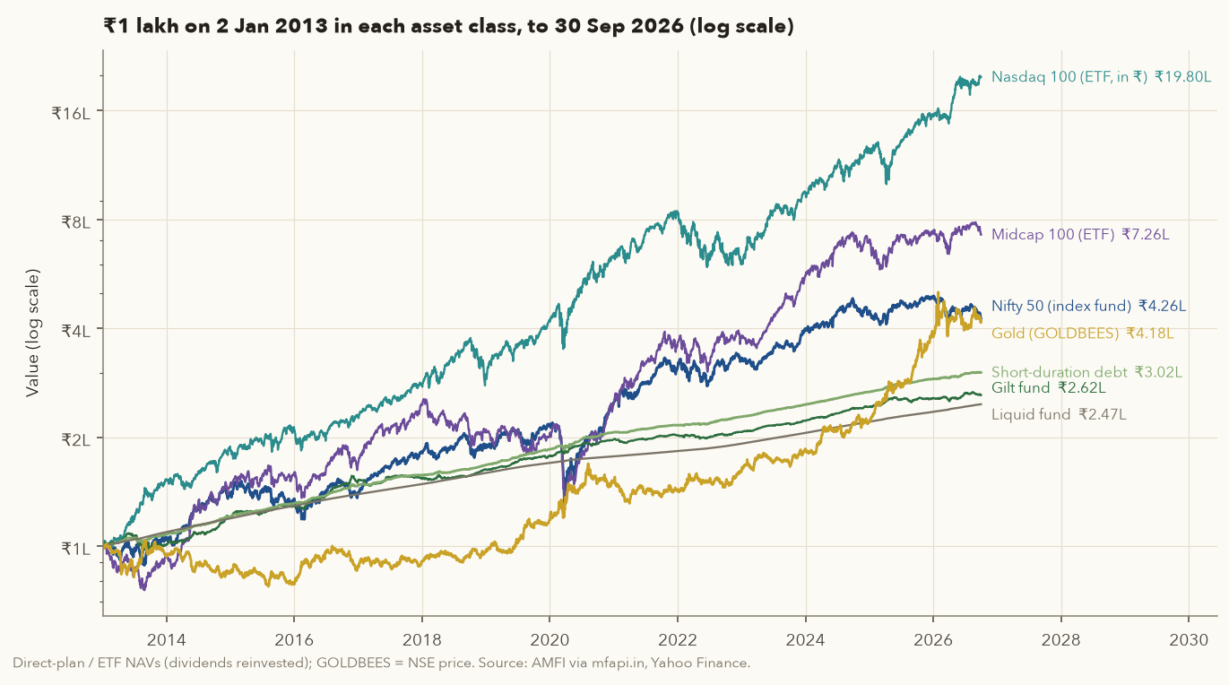
Over 13¾ years to 30 Sep 2026, ₹1 lakh in a Nifty 50 index fund became ₹4.26 lakh, in gold ₹4.18 lakh, in a short-term debt fund ₹3.02 lakh and in a Nasdaq 100 ETF ₹19.80 lakh. Which assets you held, and in what proportion, decided far more than which fund house you picked. And when you change the proportions, the tax rules of chapter 15 decide how much of the gain you keep: in the backtests below, the same 60/30/10 portfolio ended with ₹1.03 crore or ₹1.09 crore after tax depending only on how it was rebalanced.
You will learn, with real NAVs to 30 Sep 2026: the long-run return, volatility, worst falls and correlations of each Indian asset class; how much each one helped in the 2020, 2022, 2024–25 and 2026 equity falls; how to size an emergency fund and fund a goal with a step-up SIP (systematic investment plan: a fixed monthly investment into a fund); the main allocation models and their weak points; whether valuation-based ("tactical") shifts helped; what hybrid funds do for you; whether rebalancing adds return or only reduces risk, before and after tax; a tax-aware rebalancing playbook with a fully worked ticket; how to write your own Investment Policy Statement; and how withdrawals in retirement interact with the order of returns.
This chapter builds on earlier ones rather than repeating them: diversification maths is in chapter 11, part 3; the market's P/E and bond yields in chapter 8, part 14; the core/satellite "three buckets" of your own framework in chapter 17, part 3; listed-equity tax in chapter 13, part 7; and the harvesting of long-term capital gains (LTCG; gains on assets held long enough to count as long-term, as opposed to short-term capital gains, STCG) in chapter 13, part 14 (for funds, chapter 15, part 10).
Every fund named here was chosen because it has a long, clean NAV history that illustrates an asset class. None is a recommendation. Tax rules are those in force for tax year 2026-27 (Income-tax Act, 2025, unchanged by Budget 2026 for fund gains); your own situation may differ, so consult a chartered accountant (CA) before acting on anything tax-related.
2. The asset classes open to an Indian investor
Varsity's asset-allocation chapter starts from a simple idea: you cannot avoid owning assets, because cash itself loses value to inflation; and since nobody can predict which asset will do best next decade, the sensible answer is to own a little of several whose returns come from different drivers. Owning five large-cap funds is not diversification. It is sometimes called "diworsification": more funds, same driver.
Here are the main classes, what drives each, and how a fund holding it is taxed. The tax class matters for rebalancing, because it decides what a sale costs you. Chapter 15, part 3 has the full rules; the short version for 2026-27 is in the last column.
| Asset class | Typical vehicle | What drives it | Tax class of the fund (2026-27) |
|---|---|---|---|
| Indian large-cap equity | Nifty 50 / Sensex index fund or ETF | Profits of India's biggest companies | Equity-oriented: ≤ 12 months 20%; > 12 months 12.5% above ₹1.25 lakh a year |
| Indian mid/small-cap equity | Midcap 150, Smallcap 250 index funds; active funds | Same, with more growth and more risk | Equity-oriented (same as above) |
| International equity | Nasdaq 100 or S&P 500 ETF, or a fund of funds (FoF) | Foreign company profits and the rupee–dollar rate | Not equity-oriented: listed ETF long-term after 12 months, FoF after 24; long-term 12.5%, short-term at your slab |
| Debt: liquid / overnight | Liquid fund | Short-term interest rates | Specified mutual fund (a fund with more than 65% in debt and money-market instruments; units bought from 1 Apr 2023): slab rate always, however long you hold. Older units: 12.5% after 24 months |
| Debt: short duration | Short-duration or corporate-bond fund | Interest rates and (small) credit risk | Specified mutual fund: slab rate always |
| Debt: gilt / long duration | Gilt fund, G-sec ETF | Interest-rate changes: prices rise when rates fall | Specified mutual fund: slab rate always |
| Debt you already own | EPF (8.25% for 2025-26), PPF (7.1% for Oct–Dec 2026) | Government-set rates | Not market-taxed; PPF interest is tax-free, EPF interest on employee contributions above ₹2.5 lakh a year is taxable |
| Gold / silver | Gold or silver ETF; gold FoF; Sovereign Gold Bonds (SGBs, no new issues since 2024) | Global metal prices and the rupee | ETF long-term after 12 months, FoF after 24; long-term 12.5%, short-term at slab. SGB redemption gain is exempt only for original subscribers who hold to maturity (Budget 2026) |
| Real estate | Your house; listed REITs | Rents and property values | REIT units: long-term after 12 months, 12.5% above the same ₹1.25 lakh exemption; distributions are taxed by their type |
| Cash | Savings account, sweep FD | Bank deposit rates | Interest taxed at slab |
Three points beginners miss:
- Your EPF, PPF and house are part of your allocation. If ₹8 lakh of your ₹20 lakh of savings is in EPF and PPF, you already hold 40% "debt" before you buy a single debt fund.
- Debt is there to be stable, not to earn the most. Varsity's review chapter advises sticking to high-quality (government and AAA) bonds and short-to-intermediate maturities, and avoiding credit-risk funds unless you are an expert in debt. Chapter 14, part 8 explains duration and credit risk.
- International equity diversifies two ways: different companies (US markets are dominated by technology, India's by financials and older-economy businesses), and a different currency. When the rupee weakens, rupee returns on a US fund go up.
Two smaller classes, measured on real data: the Nippon India Silver ETF returned 30.4% a year from its launch on 4 Feb 2022 to 30 Sep 2026, but with a 44.4% fall along the way and 37% annual volatility. Embassy Office Parks REIT, India's first REIT, returned 10.85% a year from 1 Apr 2019 including distributions (Yahoo's distribution-adjusted price), with a 33% maximum fall. Both are optional extras; neither is needed for a sound plan.
3. Thirteen years of real data: return, risk and drawdowns
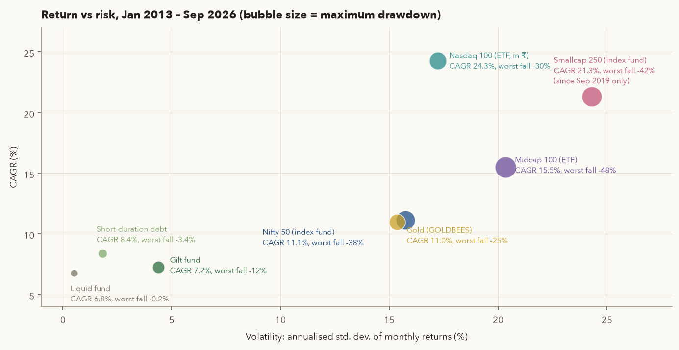
To compare asset classes fairly, we use one fund per class with a daily NAV history from 2 Jan 2013 (when "direct" plans began) to 30 Sep 2026: 13.74 years. A fund's NAV (net asset value per unit, defined in chapter 14) already includes reinvested dividends and is net of the fund's expenses, so it is the return you would actually have had. The funds are listed in the Sources.
Four measures, each defined once:
- CAGR (compound annual growth rate): the steady yearly rate that turns the start value into the end value, \( \text{CAGR} = (V_{end}/V_{start})^{1/\text{years}} - 1 \). See chapter 1.
- Volatility: the standard deviation of monthly returns, scaled to a year by multiplying by \( \sqrt{12} \). It measures how bumpy the ride is.
- Maximum drawdown: the largest fall from a previous peak to a later low, on daily NAVs. It measures how bad it can feel.
- Worst 12-month and worst 3-year return (annualised), from month-end NAVs: the worst outcome for someone who needed the money after one or three years.
| Asset (fund) | CAGR | Volatility | Max drawdown | Worst 12 months | Worst 3 years (a year) | ₹1 lakh became |
|---|---|---|---|---|---|---|
| Nifty 50 (UTI Nifty 50 Index Fund) | 11.1% | 15.7% | −38.4% | −25.4% | −1.1% | ₹4.26 L |
| Midcap 100 (Motilal Oswal ETF NAV) | 15.5% | 20.3% | −48.4% | −34.7% | −11.6% | ₹7.26 L |
| Nasdaq 100 in rupees (Motilal Oswal ETF NAV) | 24.3% | 17.2% | −30.1% | −25.8% | +11.7% | ₹19.80 L |
| Gold (GOLDBEES price) | 11.0% | 15.4% | −25.5% | −15.3% | −7.8% | ₹4.18 L |
| Gilt fund (HDFC Gilt) | 7.2% | 4.4% | −11.9% | −0.6% | +3.8% | ₹2.62 L |
| Short-duration debt (ICICI Pru Short Term) | 8.4% | 1.8% | −3.4% | +3.7% | +6.0% | ₹3.02 L |
| Liquid fund (SBI Liquid) | 6.8% | 0.5% | −0.2% | +3.2% | +4.1% | ₹2.47 L |
| Smallcap 250 (Motilal Oswal index fund), from 11 Sep 2019 only | 21.3% | 24.3% | −42.4% | −9.0% | +13.5% | n/a |
How to read these numbers
- The past decade is one sample. The Nasdaq 100's 24.3% a year combined a historic US tech boom with a weaker rupee: the dollar went from ₹54.68 to ₹96.05 over the period, 4.2% a year, and every rupee of that is in the ETF's return. Planning on it repeating is how people get hurt. Varsity's own planning chapters use deliberately conservative assumptions (about 10–11% for equity), and so will we in part 7.
- Gold is not a steady asset. It lost money in 2013, 2014 and 2015 (−6.6%, −9.3%, −7.5%), was below its January 2013 level until 2019, then gained 71.8% in 2025 alone. Its 11.0% CAGR depends heavily on the end date.
- Debt funds can fall. The gilt fund dropped 11.9% from its peak when interest rates rose. Only liquid and short-duration funds were close to "always up".
- Worst 3-year returns tell you the honest minimum horizon: the Nifty 50 fund still lost money over some 3-year windows (−1.1% a year) and the midcap ETF lost 11.6% a year. Money you need within three years does not belong in equity.
4. Correlation, and what each asset did in four falls
Correlation (ρ, "rho") measures how two assets' returns move together, from +1 (always together) through 0 (unrelated) to −1 (always opposite); chapter 11 has the maths. Diversification works when you combine assets with low or negative correlation, because one's bad months are partly offset by the other's.
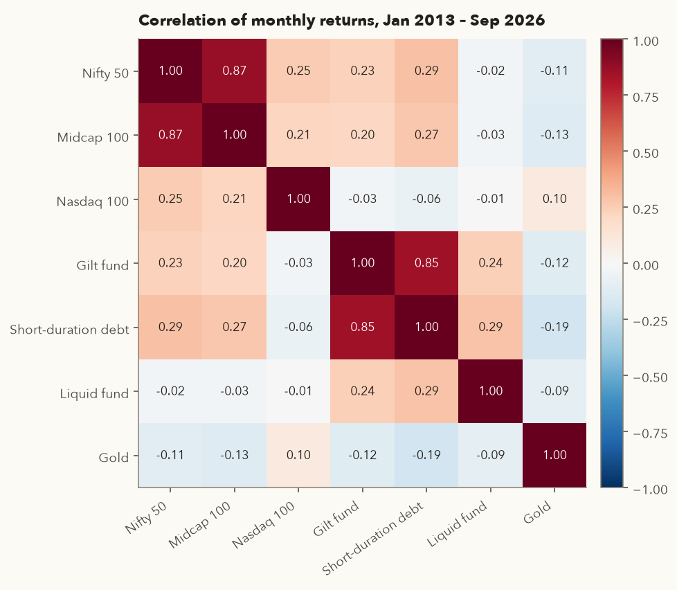
The formula from chapter 11 shows why gold helps despite being as volatile as the Nifty. For two assets with weights \(w_1, w_2\), volatilities \(\sigma_1, \sigma_2\) and correlation \(\rho\):
- \(w_1,\ w_2\)
- The share of the portfolio in asset 1 and asset 2, as fractions that add up to 1 (90% = 0.9).
- \(\sigma_1,\ \sigma_2\)
- ("sigma") Each asset's volatility: the annualised standard deviation of its returns, as a fraction (15.75% = 0.1575).
- \(\rho\)
- ("rho") The correlation between the two assets' returns, from −1 to +1.
- \(w_1^2\)
- The small 2 means "squared": the number times itself (\(0.9^2 = 0.81\)).
- \(\sqrt{\ \ }\)
- The square root: the number that, multiplied by itself, gives what is under the sign.
- \(\sigma_p\)
- The volatility of the whole portfolio, as a fraction (×100 for %).
- Square each weight times its volatility and add the two: the risk each asset brings on its own.
- Add the cross term \(2\,w_1 w_2\,\rho\,\sigma_1\sigma_2\). With positive \(\rho\) it adds risk; with \(\rho\) near zero it adds almost nothing; with negative \(\rho\) it subtracts risk.
- Take the square root of the total. Only when \(\rho = 1\) does the answer equal the weighted average of the two volatilities; anything lower gives you less. The Nifty + gold example below works it through.
Adding 10% gold to a Nifty portfolio
- Inputs measured above: \( \sigma_N = 15.75\% \), \( \sigma_G = 15.36\% \), \( \rho = -0.11 \); weights 90% Nifty, 10% gold.
- \( 0.9^2 \times 0.1575^2 = 0.81 \times 0.024806 = 0.020093 \)
- \( 0.1^2 \times 0.1536^2 = 0.01 \times 0.023593 = 0.000236 \)
- \( 2 \times 0.9 \times 0.1 \times (-0.11) \times 0.1575 \times 0.1536 = -0.000479 \)
- Sum = 0.019850, so \( \sigma_p = \sqrt{0.019850} = 14.09\% \). If gold had moved in lockstep with the Nifty (ρ = 1), the answer would have been the weighted average, 15.71%. The low correlation removed about 1.6 points of volatility for free.
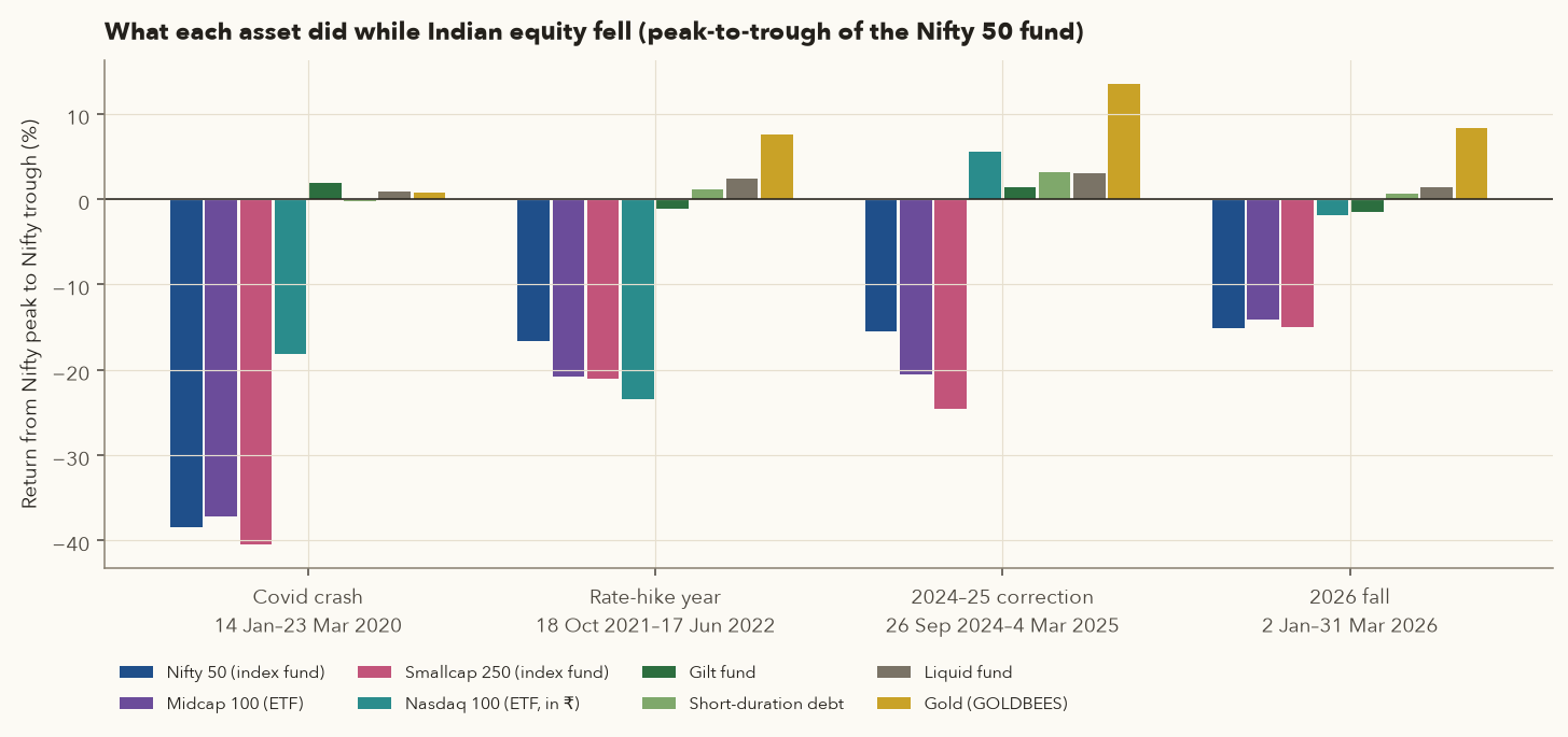
Correlations are averages, and they change. What matters most is what an asset does when you need it: in a sharp equity fall. The chart measures each fund from the Nifty 50 fund's peak to its trough in the four falls of the last seven years.
| Fall (Nifty 50 fund peak → trough) | Nifty 50 | Midcap 100 | Smallcap 250 | Nasdaq 100 | Gilt | Short debt | Gold |
|---|---|---|---|---|---|---|---|
| Covid: 14 Jan → 23 Mar 2020 | −38.4% | −37.2% | −40.5% | −18.1% | +1.9% | −0.2% | +0.8% |
| Rate hikes: 18 Oct 2021 → 17 Jun 2022 | −16.6% | −20.8% | −21.1% | −23.4% | −1.1% | +1.2% | +7.6% |
| Correction: 26 Sep 2024 → 4 Mar 2025 | −15.5% | −20.5% | −24.6% | +5.6% | +1.5% | +3.1% | +13.6% |
| 2026: 2 Jan → 31 Mar 2026 | −15.1% | −14.1% | −14.9% | −1.9% | −1.5% | +0.7% | +8.4% |
- Mid and small caps fall at least as hard as large caps in a crash. They are more equity, not a diversifier.
- International equity is not a hedge: in March 2020 and in 2022 it fell with India; in 2024–25 and 2026 it held up. Over the whole calendar year 2022 the Nasdaq 100 ETF lost 25.8% in rupees while the Nifty 50 fund made 5.4%. It diversifies across years more than across crashes.
- Gold was the most reliable cushion in these four episodes, and short-duration debt the most reliable "dry powder" (money ready to buy equity cheaply).
- Varsity's warning stands: as more assets become easily traded (ETFs, leverage), correlations can rise exactly when you need them low. Diversification lowers risk; it does not remove it.
Why not let an optimiser pick the "best" mix?
Varsity's Module 9 shows how to use the same formula, extended to many assets with a correlation matrix, to find the mix with the highest expected return for a given risk: portfolio optimisation, which traces the "efficient frontier". We tried it with Nifty 50, Midcap 100, Nasdaq 100, short-term debt and gold, using past average returns as the "expected" returns and asking for the best mix at the volatility of a 60/30/10 portfolio (no short selling):
- 2013–2026 data: 0% Nifty 50, 14% midcap, 48% Nasdaq 100, 25% debt, 13% gold.
- 2013–2019 data only: 0% Nifty, 10% midcap, 53% Nasdaq, 38% debt, 0% gold.
- 2020–2026 data only: 0% Nifty, 17% midcap, 32% Nasdaq, 11% debt, 41% gold.
The optimiser simply loads up on whatever did best in the sample it was given, and its answer swings wildly when the sample changes (gold from 0% to 41%). The 2013–2019 answer happened to keep working, because the Nasdaq kept winning; nobody could have known that in 2020. Optimisers are very sensitive to the expected returns you feed them, and those are exactly what nobody can forecast. For a personal portfolio, round and robust weights you can stick with (part 8) beat "optimal" weights estimated from one decade.
5. Why allocation drives most of the outcome
A portfolio's return is the weighted sum of its parts, which Varsity's retirement chapter calls the "sum product":
- \(i\)
- Each asset in the portfolio (here: Nifty fund, short-term debt fund, GOLDBEES).
- \(w_i\)
- The weight of asset \(i\): its share of the portfolio, as a fraction. The weights add up to 1.
- \(R_i\)
- The return of asset \(i\), in % a year (here, each fund's CAGR from part 3).
- \(\sum_i\)
- "Add up over every asset" (capital sigma means "sum").
- \(R_p\)
- The portfolio's return, in % a year.
How it works: multiply each asset's return by its weight and add the results: a weighted average (Excel's SUMPRODUCT). In the example, 60% of the money earned 11.12%, 30% earned 8.37% and 10% earned 10.96%, giving 6.67 + 2.51 + 1.10 = 10.28% a year.
That is the weighted average of the three CAGRs above, for a 60/30/10 mix of the Nifty fund, the short-term debt fund and GOLDBEES. (The realised CAGR of the actual portfolio differs a little, depending on rebalancing; see part 12.) Risk, by contrast, is less than the weighted average: the same mix had a volatility of 9.59% computed from the measured correlations, against a weighted average of the three volatilities of 11.53%.
The famous "90%" claim, and its caveats
In 1986 Brinson, Hood and Beebower studied 91 large US pension funds over 1974–1983 and found that the policy mix (how much in shares, bonds and cash) explained 93.6% of the variation in each fund's quarterly returns over time. Stock selection and market timing explained little. This is often repeated as "asset allocation explains 90% of returns". In 2000 Ibbotson and Kaplan clarified what the number means:
- About 90% of the ups and downs of one portfolio over time come from its allocation, mostly because all portfolios rise and fall with the markets they hold.
- Only about 40% of the differences between two investors' returns is explained by their different allocations; fund choice, costs and timing explain the rest.
- On average about 100% of the return level comes from the allocation, because active choices, after costs, roughly cancel out.
The practical lesson: get the big split right first, keep costs low, and do not expect fund-picking to rescue a wrong allocation. Varsity's review chapter puts it in one line: asset allocation, risk management and behaviour determine your returns, not picking the "best fund".
6. Risk capacity, tolerance and need; the emergency fund first
Three different questions decide how much equity you should hold. Planners keep them separate:
| Concept | Question | What raises it |
|---|---|---|
| Risk capacity | How big a loss can your finances absorb without derailing a goal? | Long horizon, stable income, emergency fund in place, few dependants, no high-interest debt |
| Risk tolerance | How big a fall can you watch without selling in panic? | Experience of past falls, understanding of what you own |
| Risk need | How much return do your goals require? | Big goals relative to savings, short time |
Your equity share should respect the lowest of the three. A 25-year-old with a secure job has high capacity, but if she sold everything in March 2020 her tolerance was lower than her plan. Someone who has already saved enough for retirement has low need and gains little from taking more risk. Your human capital (the present value of your future earnings, which Varsity's review chapter calls your biggest asset) matters too: a salaried government employee's income behaves like a bond, so she can hold more equity; a trader or business owner whose income already depends on markets should hold less.
A quick test of tolerance using part 3: in early 2020 the Nifty 50 fund fell 38.4% in ten weeks. With ₹10 lakh in a 60/30/10 portfolio, the equity part would have gone from ₹6 lakh to about ₹3.7 lakh. If that thought makes you want to sell, lower the equity share now, while markets are calm.
The emergency fund comes before any allocation
Varsity's portfolio chapter makes two assumptions before building any fund portfolio: you have term life and health insurance, and you have an emergency fund, money for job loss, repairs or hospital deposits that you can reach in a day. Common advice is 3 to 12 months of expenses: fewer if your job is secure and you are young, more if your income is irregular. Varsity's point is that liquidity matters more than return here, and that you can build it up with a SIP rather than all at once.
Where to keep it: part in your savings account, the rest in a liquid fund (a debt fund holding instruments of up to 91 days). Many liquid funds offer instant redemption of up to ₹50,000 (or 90% of the holding, if lower) per day, and liquid funds charge only a tiny exit load for the first six days.
Six months' expenses in a liquid fund
- Expenses ₹60,000 a month × 6 months = ₹3,60,000.
- NAV rose from ₹4,182.7123 to ₹4,452.8811: return = 4,452.8811 / 4,182.7123 − 1 = 6.46%, or ₹23,253 on ₹3.6 lakh.
- Liquid-fund gains are taxed at your slab rate (a specified mutual fund). At 30% plus 4% cess (31.2%) you keep ₹15,998, or 4.44% after tax. At a lower slab you keep more.
- Many large banks pay 2.5–3% on savings balances (check yours), also taxed at slab. The liquid fund is not "risk-free" (it holds short-term debt), but it has been the steadiest asset in this chapter: its worst fall since 2013 was 0.2%.
The emergency will not wait for the market to recover. Count the emergency fund outside your allocation, and do not rebalance it into anything.
7. Goal-based buckets and a worked goal plan
Varsity defines a financial goal by three things: the amount needed, the time available and your age (which signals how much risk you can carry). Instead of one big portfolio, many investors keep a bucket per goal, each with an allocation that suits its deadline:
| Time to goal | Sensible home | Why (from part 3) |
|---|---|---|
| Under 3 years | Liquid, money-market or short-duration debt funds; FDs | Equity lost money over some 3-year windows |
| 3 to 7 years | Mostly debt with some equity (for example 30–40%), or a conservative hybrid fund | Equity's worst 12 months were −25% to −35%; the debt part has to cover the goal if equity is down |
| Over 7 years | Mostly equity (60–80%), some debt and gold; move to debt as the date nears (a "glide path", part 8) | Long windows smoothed out the crashes |
Two formulas from chapter 8's time-value-of-money section do all the work. First, inflate today's cost to the goal date at the goal's own inflation rate (education and healthcare usually run above general inflation):
- \(PV\)
- Present value: what the goal would cost today, in ₹.
- \(\pi\)
- ("pi", here just a name for inflation, not 3.14) The yearly inflation rate expected for this goal, as a fraction (8% = 0.08).
- \(n\)
- Years until the goal.
- \((1+\pi)^{n}\)
- \((1+\pi)\) multiplied by itself \(n\) times: prices rising by \(\pi\) every year, compounded.
- \(FV\)
- Future value: what the goal will cost on the date you need the money, in ₹.
How it works: each year the cost grows by the inflation rate, so after \(n\) years it has been multiplied by \((1+\pi)\) \(n\) times. In the worked plan below, ₹20 lakh at 8% for 12 years becomes 20,00,000 × 1.0812 = ₹50,36,340.
Then find the monthly SIP that grows to that amount. With a monthly rate \( i = (1+r)^{1/12} - 1 \) for an expected yearly return \( r \), and \( N \) monthly instalments paid at the start of each month:
- \(FV\)
- The amount you need on the goal date, in ₹ (from the formula above).
- \(r\)
- The expected yearly return of the portfolio, as a fraction (8.55% = 0.0855).
- \(i\)
- The matching monthly return: \(i = (1+r)^{1/12} - 1\). The power \(1/12\) is the "12th root": the monthly rate that, compounded 12 times, gives \(r\) for the year.
- \(N\)
- The number of monthly instalments (12 per year: 144 for 12 years).
- SIP
- The fixed monthly amount to invest, in ₹, paid at the start of each month.
- Convert the yearly return to a monthly one, \(i\).
- \(\big[(1+i)^{N} - 1\big]/i\) is what ₹1 a month grows to after \(N\) months. The extra \((1+i)\) adds one more month of growth, because each instalment is paid at the start of its month.
- Divide the goal by that growth factor to get the monthly amount. The worked plan below gets ₹20,469 a month for ₹50.36 lakh in 12 years at 8.55%.
A step-up SIP raises the instalment by a fixed percentage each year, in line with your pay. Varsity's review chapter shows why this matters: a ₹10,000 SIP growing 10% a year at 9% beats a flat ₹10,000 SIP at 13% over 30 years. Your savings rate, which you control, matters more than the return, which you do not.
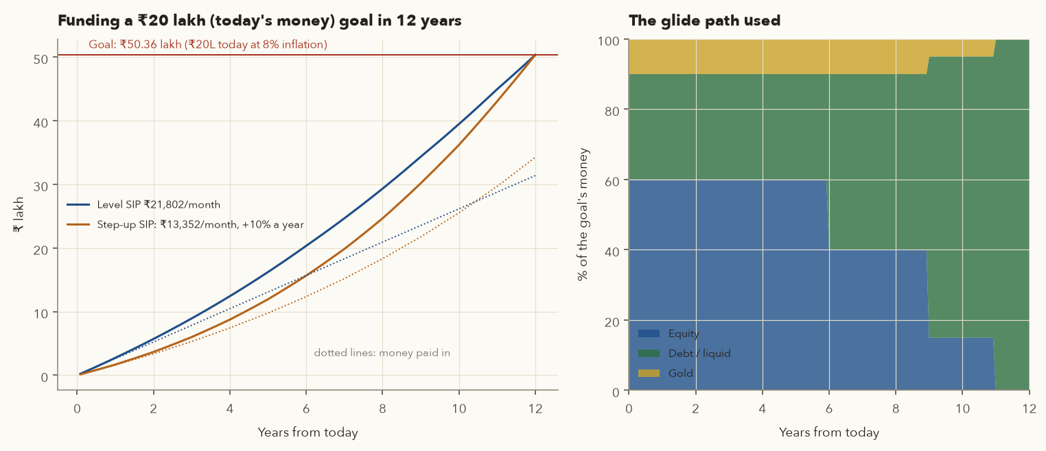
₹20 lakh in today's money, 12 years away
- Inflate: education inflation assumed 8%. \( FV = 20{,}00{,}000 \times 1.08^{12} = 20{,}00{,}000 \times 2.51817 = ₹50{,}36{,}340 \).
- Assume conservative returns (pre-tax, below the historical figures in part 3): equity 10%, debt 6.5%, gold 6%, liquid 6%. A 60/30/10 mix then expects \( 0.6 \times 10 + 0.3 \times 6.5 + 0.1 \times 6 = 8.55\% \) a year.
- Level SIP at a constant 8.55%: \( i = 1.0855^{1/12} - 1 = 0.686\% \); \( (1+i)^{144} = 2.6764 \). SIP = 50,36,340 × 0.00686 / (1.6764 × 1.00686) = ₹20,469 a month.
- With a glide path (60/30/10 until 6 years before, then 40/50/10, then 15/80/5 in the last three years, all liquid in the last year), the expected return falls as the date nears (8.55% → 7.85% → 7.0% → 6.0%), so the SIP has to be a little higher: ₹21,802 a month (₹31.39 lakh paid in over 12 years). That is the price of safety.
- With a 10% yearly step-up on the same glide path: start at ₹13,352 a month, rising to ₹38,095 in year 12 (₹34.26 lakh paid in). Easier to start; more paid in total, because later money has less time to grow.
course/scripts/ch16_figures.py.- One goal, one bucket, one spreadsheet row: amount today, inflation, date, allocation, SIP. Name the folios or tag the holdings by goal.
- Use conservative return assumptions. If markets do better, you finish early or contribute less later.
- Retirement uses the same method; Varsity's retirement chapters show that an expense of ₹50,000 a month 25 years away, at 5% inflation, needs a corpus of several crores. Start early: time is the lever you cannot buy later.
8. Allocation models: age rules, fixed mixes, glide paths, core-satellite
Age-based rules ("100 minus age")
The old rule says hold (100 − your age)% in equity: 70% at 30, 40% at 60. It is easy, and it captures one truth: your horizon shortens as you age. Its weaknesses: it ignores your goals (a 30-year-old saving for a house in 3 years should not hold 70% equity for that goal), your other assets (EPF, a paid-off house, a pension), your income stability and your tolerance. With longer lifespans some use "110 or 120 minus age". Treat any of them as a starting point, then adjust for parts 6 and 7.
Fixed strategic mixes
A strategic allocation is a long-term target you keep through good and bad markets, such as 60/30/10 equity/debt/gold. Varsity's beginner advice for anyone unsure is simple: a few big, liquid classes (a large-cap index fund, a mid-cap fund, US equity via a cheap S&P 500 fund, a short-term government/PSU bond fund, gold, perhaps REITs), with roughly equal or sensible weights, and then stick to it. The value of a fixed mix is behavioural: it is a decision made calmly, in advance.
Glide paths and SEBI's Life Cycle Funds
A glide path lowers equity on a schedule as a goal approaches, which protects the corpus against a crash just before you need it (the "sequence risk" of part 18). Varsity's portfolio chapter suggests starting to move a 10-year goal's money into debt from about year 8. In February 2026 SEBI created a new fund category that does this for you: Life Cycle Funds, target-date funds of 5 to 30 years (in multiples of 5) that must follow a prescribed glide path, and that replace the old "solution-oriented" retirement and children's funds (which stopped taking new money).
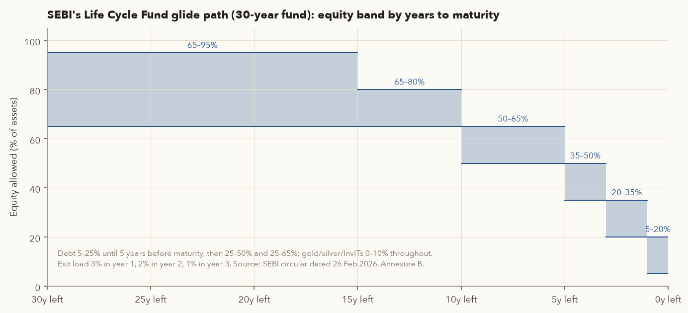
Two features to note: an exit load of 3% in the first year, 2% in the second and 1% in the third, to discourage early exits; and the fund's internal shifts from equity to debt are not taxable events for you. How the fund itself is taxed on your exit depends on its average equity share, which falls over time; check the factsheet's tax note, and see chapter 15.
Core-satellite
A core-satellite portfolio keeps most money (the core, say 80–90%) in a low-cost, diversified, rebalanced allocation, and a small part (the satellite) for active ideas: stock picks, a sector bet, or your swing-trading account. This is exactly the structure of your framework's three buckets in chapter 17, and the reason for the portfolio-heat and correlation limits in chapter 11. The core's allocation is decided by this chapter; the satellite's size is capped so that its failure cannot hurt a goal.
9. Tactical allocation using valuations, tested honestly
Tactical asset allocation means moving away from your strategic mix for a while based on a view, for example holding more equity when the market looks cheap and less when it looks expensive. Chapter 8 showed that the Nifty 50 P/E (price-to-earnings ratio) has some link with the next year's return, and warned that its history is short: NSE switched to consolidated earnings on 31 Mar 2021, so only the series since April 2021 is comparable.
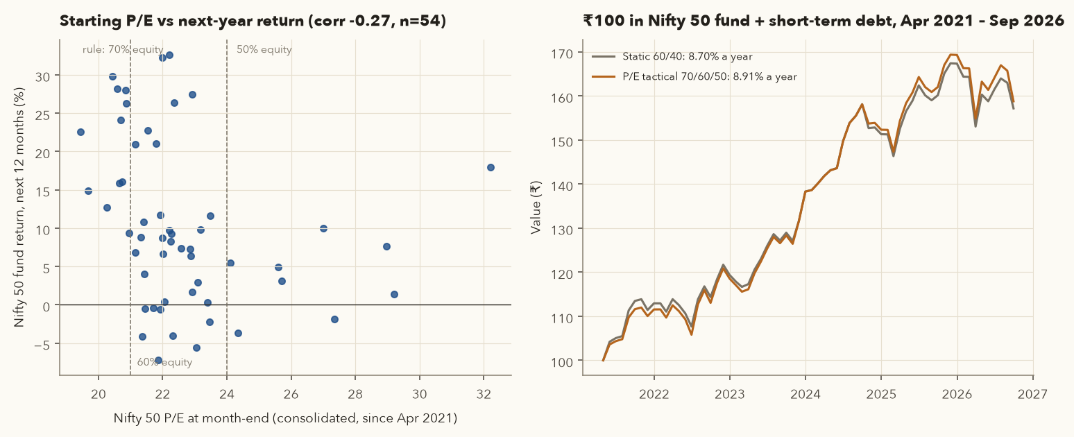
We tested a simple rule on that comparable period: hold 70% equity when the P/E at the previous month-end was below 21, 60% between 21 and 24, and 50% above 24, the rest in the short-term debt fund, rebalanced monthly. The static alternative is a constant 60/40.
A small edge, four times the trading, too little data
- The P/E rule returned 8.91% a year against 8.70% for static 60/40. The average equity weight was 61.2%; the rule spent 17 of 65 months at 70% and 9 at 50%.
- It moved 92% of the portfolio between equity and debt over the period (sum of the monthly weight changes), against 22% for monthly rebalancing of the static mix. In a taxable account every shift out of equity is a sale; in years when equity gains are above ₹1.25 lakh that costs 12.5–20%, which could eat the 0.21-point edge.
- Five and a half years, one rule, thresholds chosen after looking at the data: this is exactly the kind of result chapter 12 warns can be luck or overfitting.
If you want a valuation tilt, keep it small (±10 points around your strategic weight), decide the rule in advance, write it into your Investment Policy Statement (part 17), and carry it out mainly by steering new money, not by selling. Varsity's review chapter suggests a gentler version: when rebalancing back into equity after a fall, put more of it into the sub-class that has fallen most.
10. Hybrid funds: rebalancing done for you
A hybrid fund holds more than one asset class inside one scheme, and the fund manager keeps the mix in range. SEBI's categorisation circular of 26 Feb 2026 sets the ranges:
| Category | SEBI's rule (Feb 2026) | Usual tax class for you |
|---|---|---|
| Conservative hybrid | Equity 10–25%, debt 75–90% | Specified mutual fund (more than 65% debt): slab rate |
| Balanced hybrid | Equity 40–60%, debt 40–60%, no arbitrage | "Other": long-term after 24 months at 12.5%, short-term at slab |
| Aggressive hybrid | Equity 65–80%, debt 20–35% | Equity-oriented |
| Balanced advantage / dynamic asset allocation (BAF) | Equity and debt managed dynamically, often by a valuation model | Usually equity-oriented: most keep at least 65% gross equity by holding hedged (arbitrage) positions. Check the factsheet. |
| Multi-asset allocation | At least 10% in each of at least three asset classes (foreign shares are not a separate class) | Depends on the average equity share: equity-oriented if at least 65% domestic equity, otherwise usually "other". Check the factsheet. |
| Equity savings | At least 65% equity including arbitrage; net equity 15–40%; at least 10% debt | Equity-oriented |
The big advantage is tax: the fund's internal rebalancing is not a sale by you, so it creates no capital gain in your hands. You pay tax only when you redeem, under the fund's tax class. If a BAF qualifies as equity-oriented, you get equity taxation on what is effectively a mix of equity and debt, which is often better than holding a debt fund taxed at slab. The disadvantages: one manager's model controls your risk, the expense ratio is higher than a DIY index-fund mix, and you cannot see or control the exact allocation.
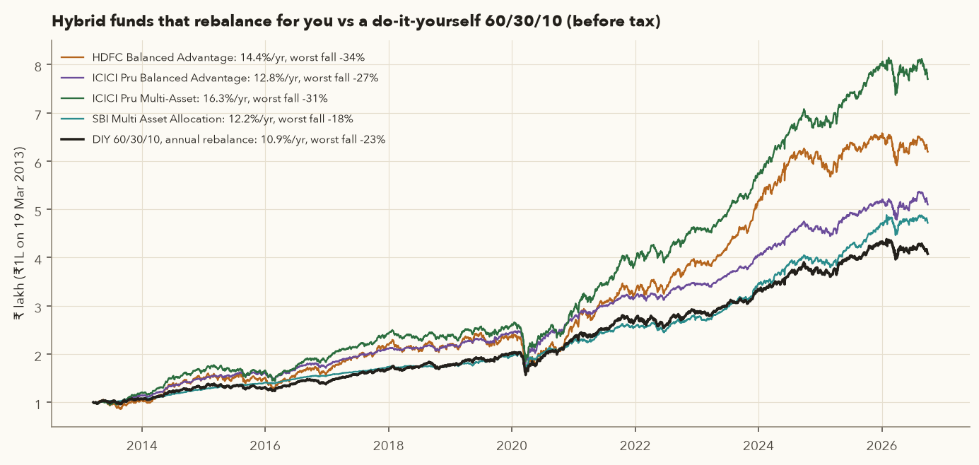
| 19 Mar 2013 → 30 Sep 2026 (direct plans) | CAGR | Volatility | Max drawdown | Worst 12 months |
|---|---|---|---|---|
| HDFC Balanced Advantage | 14.4% | 15.0% | −34.2% | −24.8% |
| ICICI Pru Balanced Advantage | 12.8% | 9.4% | −27.0% | −13.1% |
| ICICI Pru Multi-Asset | 16.3% | 12.8% | −30.6% | −20.8% |
| SBI Multi Asset Allocation | 12.2% | 6.6% | −17.6% | −1.6% |
| DIY 60/30/10 (index fund, short-term debt, GOLDBEES), annual rebalance | 10.9% | 9.3% | −23.2% | n/a |
Read this table carefully, because the obvious conclusion ("hybrids win") is not safe:
- Selection bias. These are four large, surviving funds chosen because they have long histories. Weaker hybrid funds that were merged or closed are not in the list.
- "Balanced" names hide very different risk. HDFC Balanced Advantage fell 34.2% at its worst, which is close to the Nifty's 38.4%. SBI Multi Asset fell only 17.6%. Compare the drawdown, not the label.
- Different ingredients. The hybrids held active stock picks, mid caps and (in multi-asset funds) commodities and arbitrage; the DIY mix held only the Nifty 50. Part of their lead is active management having a good decade, which the SPIVA evidence in chapter 14, part 9 says does not reliably persist.
When a hybrid fund makes sense: smaller portfolios where the simplicity is worth more than the extra expense ratio; investors who will not rebalance themselves; and debt-like allocations where the equity-oriented tax class is valuable. A BAF can be the "debt plus a bit of equity" bucket for a 3–7 year goal, for example.
11. Rebalancing: why, and three ways to do it
Left alone, a portfolio drifts: the asset that rose most takes a bigger share. Varsity's review chapter gives the example of a 60/30/10 portfolio that becomes 70/25/5 after a good year for equity. Its risk is now that of a 70% equity portfolio, which you never chose. Rebalancing means trading back towards the target: selling some of what is overweight and buying what is underweight. Two reasons to do it:
- Risk control: keep the risk you chose. This is the main reason.
- A built-in "buy low, sell high": you trim what has risen and add to what has fallen. Whether this adds return depends on whether the assets take turns (it helps) or one keeps winning (it hurts). Part 13 tests both cases.
Define the drift of asset \(i\) as its current weight minus its target weight, and the trade that restores the target:
- \(i\)
- One asset in the portfolio (equity, debt or gold).
- \(V_i\)
- Today's value of your holding in asset \(i\), in ₹.
- \(V\)
- The total value of the portfolio today, in ₹.
- \(w_i\)
- The current weight of asset \(i\): its share of the total.
- \(w_i^{*}\)
- The target weight you chose (the star marks "target"), e.g. 0.60 for 60% equity.
- \(d_i\)
- The drift, in percentage points: positive means overweight, negative underweight.
- \(\text{Trade}_i\)
- The rupees to buy (positive) or sell (negative) in asset \(i\) to get exactly back to target.
- Divide each holding by the total to get its current weight.
- Subtract the target weight: that is the drift, which your band rule checks.
- To rebalance, work out what the asset should be worth (target weight × total) and subtract what it is worth now. A positive trade is a buy, a negative one a sale. The trades add up to zero: sales pay for the buys.
Example (illustrative, using Varsity's drift): a ₹10 lakh 60/30/10 portfolio has become ₹7 lakh equity, ₹2.5 lakh debt and ₹0.5 lakh gold, i.e. 70/25/5. Equity drift = 0.70 − 0.60 = +10 points. Trades: equity 0.6 × 10,00,000 − 7,00,000 = −₹1,00,000 (sell); debt 3,00,000 − 2,50,000 = +₹50,000 (buy); gold 1,00,000 − 50,000 = +₹50,000 (buy).
The three methods
| Method | Rule | Strength | Weakness |
|---|---|---|---|
| Calendar | Back to target on a fixed date, e.g. once a year | Simple; easy to remember | Trades even when drift is tiny; the date chosen matters more than you would think (part 13) |
| Threshold (band) | Check monthly; rebalance only when an asset is outside its band | Trades only when it matters | Needs monitoring |
| Cash-flow | Send new money (SIPs, bonuses) to whatever is underweight; never sell | No tax, no exit load | Too weak once the portfolio is large relative to new money |
A common band rule is the "5/25 rule": rebalance when an asset is more than 5 percentage points away from target or more than 25% of its own target away, whichever is tighter. For 60% equity the band is 55–65% (5 points is tighter than 15). For 10% gold it is 7.5–12.5% (2.5 points is tighter than 5). Varsity's review chapter suggests an annual check with a 5% tolerance band.
Cash-flow rebalancing splits each new instalment \(C\) in proportion to how far each asset is below target after adding it:
- \(C\)
- The new money to invest this time (a SIP instalment or a bonus), in ₹.
- \(V,\ V_i,\ w_i^{*}\)
- As above: portfolio total before the new money, value in asset \(i\), and target weight of asset \(i\).
- \(w_i^{*}(V+C)\)
- What asset \(i\) should be worth once the new money is in.
- \(\max(\dots,\ 0)\)
- "The larger of the bracket and 0": how far asset \(i\) is below target, in ₹. An overweight asset scores 0, so it gets nothing.
- \(\sum_j\)
- Add up the shortfalls of every asset \(j\) (the same calculation, for all assets).
- \(\text{Buy}_i\)
- The rupees of the new money that go into asset \(i\).
- For each asset, work out its target value after adding \(C\), and how far short of that it is (zero if it is already above).
- Add up all the shortfalls.
- Give each asset its share of \(C\) in proportion to its shortfall. Nothing is sold. (If no asset is short, the framework splits \(C\) by the target weights.)
Example (illustrative, same 70/25/5 portfolio, \(C\) = ₹50,000): after adding, the total is ₹10.5 lakh. Targets: equity ₹6.3 lakh (it has ₹7 lakh, shortfall 0), debt ₹3.15 lakh (short ₹65,000), gold ₹1.05 lakh (short ₹55,000). Total shortfall ₹1,20,000. Debt gets 50,000 × 65/120 = ₹27,083; gold gets 50,000 × 55/120 = ₹22,917; equity gets nothing.
12. Does rebalancing pay? The before-tax backtest
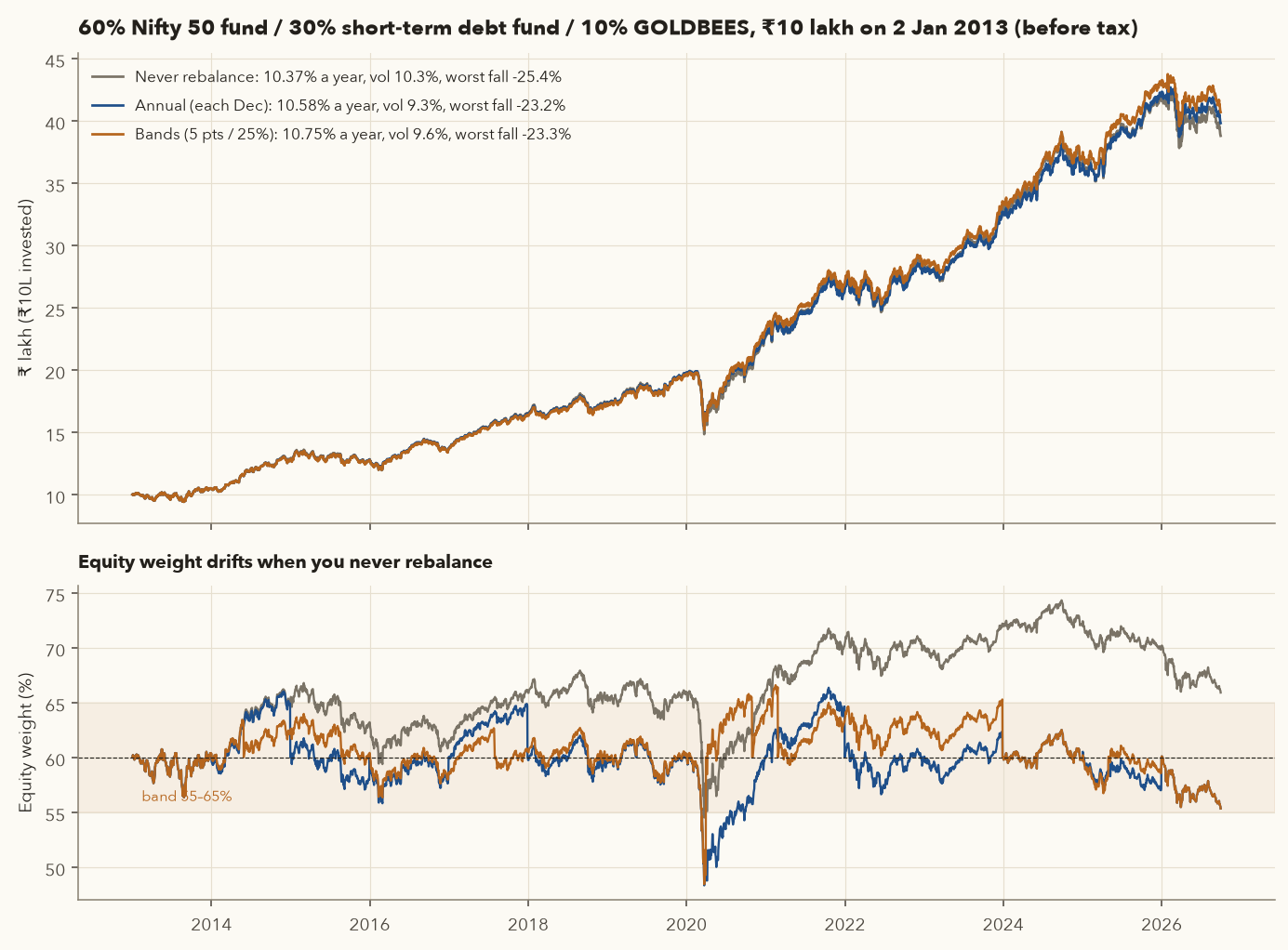
We tested a 60/30/10 portfolio built from three real funds: the UTI Nifty 50 Index Fund (direct), the ICICI Prudential Short Term Fund (direct) and GOLDBEES. ₹10 lakh was invested on 2 Jan 2013 and held to 30 Sep 2026, with the actual daily NAVs, purchase stamp duty, STT, ETF exchange charges and an assumed 0.05% spread on each ETF trade. The engine keeps every purchase as a separate lot (a batch of units bought on one date) and sells them first-in-first-out (FIFO), as the law requires (chapter 13). First, the before-tax picture:
| ₹10 lakh lump sum, before tax | Value 30 Sep 2026 | CAGR | Volatility | Max drawdown | Rebalances | Turnover a year |
|---|---|---|---|---|---|---|
| Never rebalance | ₹38.78 L | 10.37% | 10.3% | −25.4% | 0 | 0% |
| Annual, each December | ₹39.80 L | 10.58% | 9.35% | −23.2% | 13 | 2.3% |
| Bands (5 points / 25%), checked monthly | ₹40.68 L | 10.75% | 9.56% | −23.3% | 8 | 2.8% |
course/scripts/ch16_figures.py.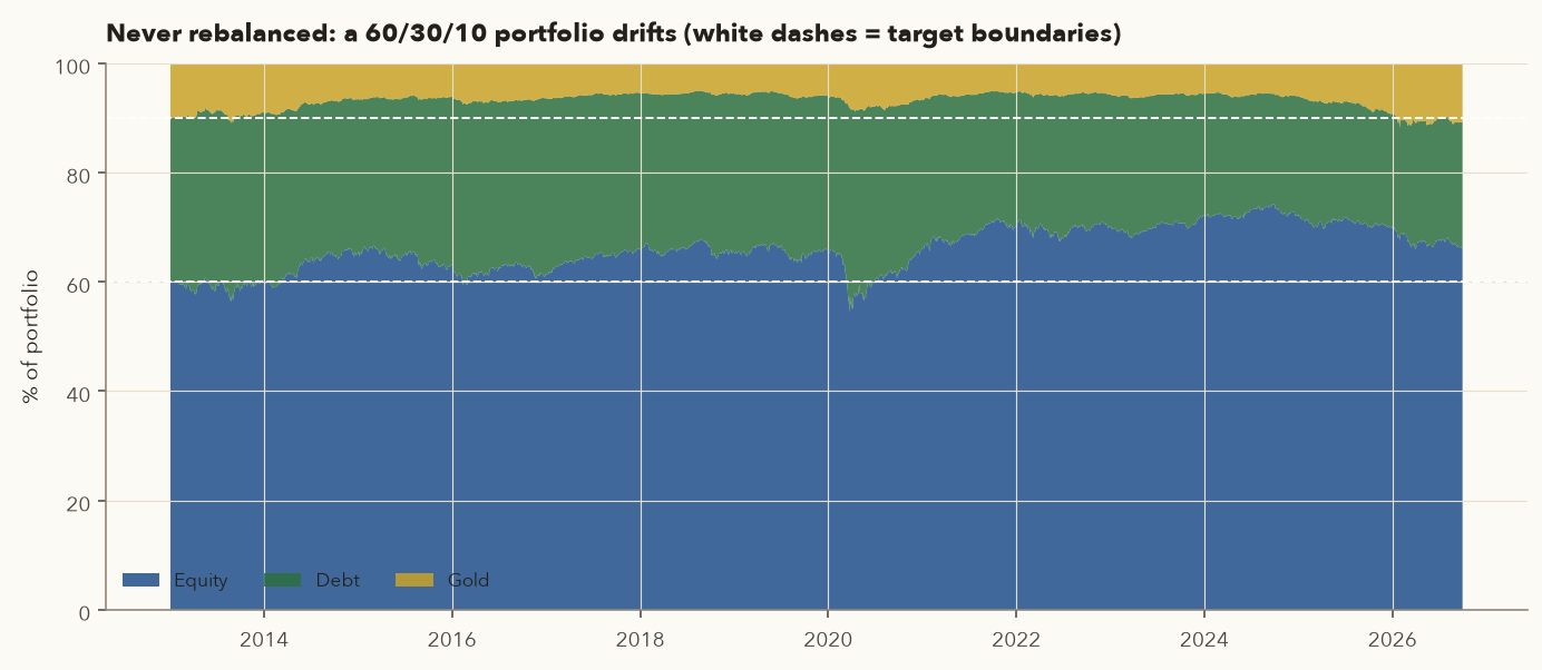
What the before-tax test says:
- Rebalancing reduced risk: volatility fell from 10.3% to about 9.4–9.6% and the worst fall from −25.4% to about −23.2%.
- It also added a little return in this sample, 0.2–0.4 points a year, because Indian equity, debt and gold took turns: gold was bought cheaply in 2013–2018 and trimmed after its rallies; equity was bought after March 2020.
- Starting in January 2015 instead gives the same ordering with smaller gaps: 10.05% (never), 10.15% (annual), 10.43% (bands) a year.
- Trading was light: 2–3% of the portfolio a year. Costs over 13¾ years were a few hundred rupees.
13. After tax and costs: five methods for a SIP investor
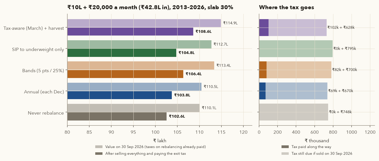
Now the realistic case: ₹10 lakh on 2 Jan 2013 plus ₹20,000 on the first trading day of every month (₹42.8 lakh paid in), a 30% slab, and every sale taxed under the 2026-27 rules from chapter 15 as if they had always applied: equity fund 20% short-term, 12.5% long-term above ₹1.25 lakh a year (with "grandfathering" for units bought before 1 Feb 2018: gains up to their 31 Jan 2018 value are not taxed); debt fund at slab for units bought from 1 Apr 2023, and 12.5% after 24 months for older units; gold ETF 12.5% after 12 months, slab before; 4% cess; losses set off and carried forward as the law allows. Tax due on a sale is paid out of the portfolio on the day. At the end we also compute the exit tax: what you would owe if you sold everything on 30 Sep 2026.
The five methods: never rebalance; annual (December); bands; cash-flow only (all SIPs to the underweight assets, never sell); and tax-aware: cash-flow SIPs, plus a check each March in which overweight assets are sold only from lots that are already long-term (and equity only up to the year's unused ₹1.25 lakh exemption), plus harvesting of equity LTCG up to the exemption each March (sell, buy back the next day; chapter 13).
| ₹10 L + ₹20,000/month, 30% slab | Rebalances | Tax paid along the way | Value 30 Sep 2026 | Exit tax | After exit tax and costs | XIRR after tax | Volatility | Max drawdown |
|---|---|---|---|---|---|---|---|---|
| Never rebalance | 0 | ₹0 | ₹1,10,06,136 | ₹7,47,742 | ₹1,02,57,467 | 9.77% | 10.1% | −24.7% |
| Annual (December) | 13 | ₹68,827 | ₹1,10,47,989 | ₹6,70,323 | ₹1,03,76,883 | 9.90% | 9.35% | −23.2% |
| Bands (5 pts / 25%) | 8 | ₹81,601 | ₹1,13,37,702 | ₹6,99,926 | ₹1,06,36,972 | 10.17% | 9.6% | −23.2% |
| Cash-flow only | 0 | ₹0 | ₹1,12,71,936 | ₹7,94,831 | ₹1,04,75,974 | 10.00% | 9.4% | −23.2% |
| Tax-aware (March) + harvest | 3 | ₹1,02,323 | ₹1,14,89,939 | ₹6,27,721 | ₹1,08,61,503 | 10.39% | 9.6% | −23.1% |
XIRR (defined in chapter 14, part 12) is the annual return on your own cash flows. "Rebalances" counts the dates on which a sale was made to restore the mix; the cash-flow method never sells, and the tax-aware method's yearly harvests are not counted.
course/scripts/ch16_figures.py.What explains the differences, honestly
- Rebalancing taxes were small: ₹69,000–₹1.02 lakh over 13¾ years, against an exit tax of ₹6.3–7.9 lakh that every method carries. The fear that "rebalancing will kill me in tax" was not borne out for this low-turnover portfolio, partly because equity sales mostly fell inside the yearly ₹1.25 lakh exemption.
- The month you choose matters as much as the method. The same annual rule done each March instead of each December ends at ₹1,07,47,068 after tax, ₹3.70 lakh more. The chart below repeats the lump-sum test for all twelve months: before tax the result ranges from ₹39.80 lakh (December) to ₹41.89 lakh (March). That spread is luck, not skill.
- The tax-aware method's lead splits into two parts. Without the harvesting step it ends at ₹1,07,61,105, almost the same as plain March rebalancing (₹1,07,47,068) but with 3 rebalancing dates instead of 14 and less tax paid along the way (₹1.08 lakh against ₹1.26 lakh). Harvesting then adds about ₹1 lakh, mostly by lowering the exit tax from ₹7.14 lakh to ₹6.28 lakh. The harvesting is the part that reliably helps; the rest is timing.
- Cash-flow rebalancing alone kept risk almost as low as the others (9.4% volatility, −23.2% worst fall) with zero tax along the way. Its limit showed late: by 2025–26 the portfolio was over ₹1 crore and a ₹20,000 SIP could not offset gold's surge.
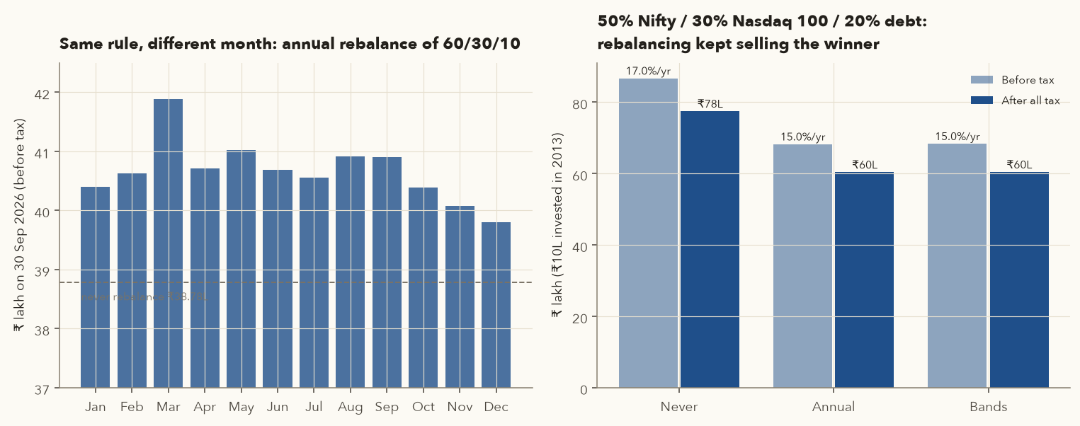
Rebalancing kept selling the winner
- ₹10 lakh in 2013. Never rebalanced: 17.0% a year, ₹86.74 lakh before tax, ₹77.52 lakh after exit tax.
- Rebalanced every December: 15.0% a year, ₹68.28 lakh before tax; ₹1.46 lakh of tax paid along the way (the Nasdaq ETF is not equity-oriented, so there is no ₹1.25 lakh exemption on its gains); ₹60.41 lakh after all tax. Bands gave almost the same result (₹60.46 lakh).
- What rebalancing bought: volatility 11.7% → 10.4%. The worst fall barely changed (−26.1% → −26.0%).
- Lesson: rebalancing is a risk-control tool. When one asset trends for a decade, it costs return. You cannot know in advance which kind of decade you are in, which is exactly why you rebalance for risk, not for profit.
14. The tax-aware rebalancing playbook
The goal is to get close to your target allocation while paying the least tax, in roughly this order of preference:
- Use new money first. Direct SIPs, bonuses and dividends to the underweight asset (cash-flow rebalancing). No sale, no tax, no exit load.
- Do not trade small drifts. Use bands (part 11) and skip any trade smaller than, say, 1% of the portfolio or ₹10,000. Small trades add work, lots and tax records for no benefit.
- Rebalance in February–March, inside the tax year's exemption. Equity sales that produce long-term gains up to ₹1.25 lakh in a tax year are tax-free (shared with your share sales; chapter 13). If you must sell equity, size the sale so that the long-term gain fits in what is left of the exemption.
- Sell long-term lots, and wait for the 12/24-month mark when it is close. FIFO decides which units go (you cannot choose lots within one folio; see chapter 15, part 5), so check the date of the oldest lot. A gold ETF lot held 11 months is taxed at your slab; once it has been held more than 12 months (exactly 12 months is still short-term, so wait a few days past the anniversary), at 12.5%. For a gold or international FoF the line is 24 months.
- Use losses. A short-term loss can absorb any capital gain; a long-term loss only long-term gains (chapter 15, part 9). If a holding is below cost, redeeming it and reinvesting in a similar but different fund banks a loss to offset the gain on what you trim. Under FIFO, losses in recent lots are stuck behind older gains in the same folio; chapter 15, part 11 shows the trap and the rules.
- Prefer trimming the asset with the lowest tax per rupee sold. Tax per rupee = (gain ÷ sale value) × rate. Equity inside the exemption: zero. A gold ETF lot that has doubled: 50% gain share × 13% = 6.5% of the sale. A post-2023 debt fund at 30% slab with a 15% gain share: 4.7%.
- Avoid exit loads. Most equity funds charge 1% if redeemed within a year; Life Cycle Funds 3/2/1%. Check before every sale.
- Consider hybrid funds for the part you would rebalance most (part 10): their internal rebalancing creates no tax for you, but check their tax class and costs.
- Think about asset location across the family (below).
- Harvest every year anyway. Even when you do not need to rebalance, book equity LTCG up to ₹1.25 lakh each March and buy back the next trading day (chapter 15, part 10). In the backtest this was the single most reliable tax saving.
Asset location across family members, and clubbing
Asset location means choosing whose name (or which account) holds each asset so the family's total tax is lowest. Each adult has a separate ₹1.25 lakh equity exemption, a separate basic exemption and slab, and a separate ₹12 lakh rebate limit for slab-rate income. Debt-fund gains are slab-rate income, so the rebate can cover them, unlike STCG/LTCG on equity (chapter 13, part 5).
Same gain, two family members
- In your hands at the 30% slab: 1,00,000 × 30% × 1.04 = ₹31,200.
- In the hands of a retired parent whose only other income is a ₹6 lakh pension: total income ₹7 lakh, below ₹12 lakh, so the rebate makes the slab tax ₹0.
- This works only if the money genuinely becomes the parent's. A gift of money from a "relative" (parents, siblings, spouse, children and others defined in the Act) is tax-free for the receiver (new s.92, old s.56(2)(x)).
Under s.99 of the new Act (old s.64), income from assets you gift to your spouse (or son's wife) without adequate consideration, and the income of a minor child (with narrow exceptions), is added to your income. So putting debt funds in a non-earning spouse's name after gifting them the money saves nothing. Gifts to adult children and to parents are not clubbed. The rules have fine print (for example, income earned on the clubbed income), so ask a CA before moving significant sums.
15. A worked rebalancing ticket on 30 Sep 2026
A "ticket" is a written record of a rebalancing decision: where you are, where you want to be, the trades, the lots, the tax and the alternative you rejected. Here is one for a portfolio built from real NAVs: ₹10 lakh invested on 1 Oct 2021 in 60/30/10 (UTI Nifty 50 Index Fund, ICICI Pru Short Term Fund, GOLDBEES), then ₹25,000 on the first trading day of each month, split 60/30/10, never rebalanced. ₹24.75 lakh paid in by 1 Sep 2026.
Step 1: where are we?
- NAV / price on 30 Sep 2026: Nifty 50 fund ₹159.2891, short-term fund ₹70.7759, GOLDBEES ₹121.59.
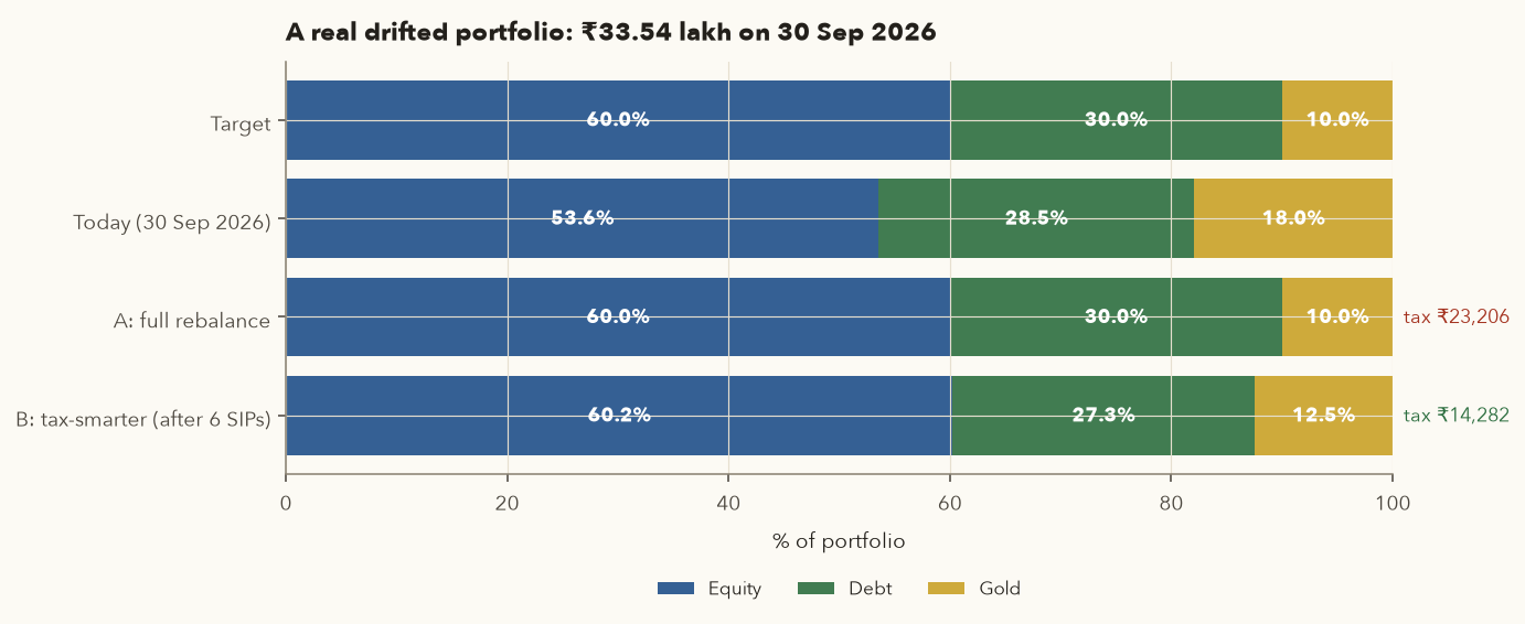
- Holdings: equity ₹17,96,436 (53.6%), debt ₹9,55,400 (28.5%), gold ₹6,02,204 (18.0%); total ₹33,54,041.
- Bands: equity 55–65% → outside (6.4 points below target); debt 25–35% → inside; gold 7.5–12.5% → outside (8.0 points above target, after gold's 71.8% rise in 2025). Action needed.
- Unrealised gains by lot. Gold: ₹3,53,255 on 48 long-term lots, ₹1,449 on 12 short-term lots. Equity: ₹3,24,981 long-term, −₹13,545 short-term (the 12 lots bought since Oct 2025, after the Nifty's 2026 fall). Debt: ₹1,69,514 on the 18 lots bought before 1 Apr 2023 (long-term, 12.5%), ₹43,387 on the 42 later lots (slab, always).
Option A: full rebalance today
- Targets: equity 60% × 33,54,041 = ₹20,12,425; debt ₹10,06,212; gold ₹3,35,404.
- Trades: sell ₹2,66,800 of GOLDBEES; buy ₹2,15,988 of the Nifty fund and ₹50,812 of the debt fund.
- FIFO: the whole sale comes from the oldest lot (1 Oct 2021, bought at ₹40.24 a unit including charges): 2,194.259 units, cost ₹88,291.83, value ₹2,66,800, long-term gain ₹1,78,508.
- Tax: 1,78,508 × 12.5% × 1.04 = ₹23,206. Gold gets no ₹1.25 lakh exemption. Charges about ₹175.
Option B: tax-smarter, nearly the same result
- Send the next six SIPs (Oct 2026 – Mar 2027, ₹1,50,000) entirely to the Nifty fund.
- Sell gold only down to the top of its band, 12.5% of the portfolio after those SIPs: sell ₹1,64,199 (1,350.4 units, same oldest lot), long-term gain ₹1,09,861, tax 1,09,861 × 13% = ₹14,282. Put the proceeds into the Nifty fund. Leave debt alone; it is inside its band.
- Allocation after the six SIPs (at today's prices): equity 60.2%, debt 27.3%, gold 12.5%. Every asset is inside its band.
- Separately, in March 2027, harvest equity: at 30 Sep 2026 prices, selling the oldest ₹4,78,544 of Nifty-fund units books exactly ₹1,25,000 of long-term gain (recompute the amount on the day), tax-free; buy back the next trading day. That removes ₹16,250 (12.5% × 1.04) of future tax.
Comparison
- Tax now: A ₹23,206, B ₹14,282, a difference of ₹8,924. Be honest about what this is: mostly deferral. The gold B keeps still carries its gain and will be taxed when sold. Deferral is still worth having, because the deferred tax keeps compounding for you.
- Risk: A is back to 60/30/10 today; B gets equity back into its band today and the rest over six months. For a long-term portfolio that difference is small.
- If gold had been held through a gold FoF instead of an ETF, lots bought within the last 24 months (not 12) would have been short-term at 31.2%, and FIFO would still have sold the oldest first.
course/scripts/ch16_figures.py.16. Implementation: one fund per asset class, and a review rhythm
Varsity's portfolio chapter warns against the "10–12 funds for one goal" portfolio (overlap is measured in chapter 14, part 14): three large-cap funds from different fund houses hold mostly the same stocks, so you pay three expense ratios for one exposure. A clean portfolio has one vehicle per asset class, sometimes two.
| Choose by | What to check (chapter 14, part 16 has the details) |
|---|---|
| Tax class | Equity-oriented vs specified debt vs "other"; ETF (12 months) vs FoF (24 months) for gold and international |
| Cost | Total expense ratio (TER, the yearly fee taken out of the NAV) of the direct plan; for ETFs, also the bid-ask spread and brokerage |
| Tracking | Tracking difference and tracking error for index funds and ETFs |
| Quality (debt) | Average maturity, credit quality (government and AAA), Macaulay duration |
| Practicalities | SIP and SWP support; exit load; ETF trading volume |
Fund or ETF?
- Index fund: easy SIPs and withdrawals on any amount, units bought at NAV, no demat needed. Stamp duty 0.005% on purchases.
- ETF: often a lower expense ratio, bought and sold on the exchange during the day, needs a demat account; stamp duty 0.015% on purchases, a small spread, and the risk of paying a premium above NAV.
An ETF premium can eat a year's return
- Closing price ₹321.08 against NAV ₹284.8257: premium = 321.08 / 284.8257 − 1 = 12.7%. On the 184 days in 2026 with both a price and a NAV, the median premium was 17.5%, and it was above 10% on 67% of them. (The NAV uses the previous US close, so single-day figures are noisy; look at the pattern, not one day.)
- Cause: limits on how much Indian funds may invest abroad stop the fund creating new units, so demand pushes the price above NAV. A buyer at a 12.7% premium loses that much if the premium disappears.
- Rule (see chapter 14, part 10): for international and thinly traded ETFs, compare the price with the indicative NAV (iNAV, published by the exchange and the fund house) before buying. If the premium is large, a fund of funds bought at NAV may be the better route despite its 24-month tax rule.
Review rhythm
- Monthly (5 minutes): SIPs went through; note the allocation.
- Quarterly: any asset outside its band? If yes, plan the rebalance (new money first).
- Yearly (February–March): harvest, rebalance, review each fund against its benchmark over 3–5 years, not 1. Varsity's review chapter suggests a red flag only if an active fund trails its benchmark by 5–10% over a short period, or after a strategy, manager or ownership change.
- On life events (marriage, child, job change, inheritance): revisit goals and risk capacity, then the allocation.
17. Your Investment Policy Statement and yearly calendar
An Investment Policy Statement (IPS) is a one-page document that records your allocation and your rules before markets test them. When the Nifty is down 15% (as in March 2026), you follow the page, not the news. Copy this template, fill in the blanks, sign and date it, and review it every April.
| Section | Fill in |
|---|---|
| Goals | Goal 1: ______ ₹____ (today's money) by ____ (year); inflation assumed __%. Goal 2: ______ … |
| Emergency fund | __ months of expenses = ₹______, held in ______ (savings / liquid fund). Not part of the allocation. |
| Risk | Largest fall I can sit through without selling: __%. Capacity notes (job, dependants, loans): ______ |
| Strategic allocation | Equity __% (India large __, mid/small __, international __); debt __% (incl. EPF/PPF? yes/no); gold __%; other __% |
| Glide path | From __ years before goal __: equity to __%; from __ years: __%; final year: all in ______ |
| Vehicles | One per class: ______ (scheme name, direct plan, tax class) |
| Contributions | SIP ₹____ a month; step-up __% each April; bonuses go to ______ |
| Rebalancing rule | Bands: ±5 points or ±25% of target, whichever is tighter. Check: quarterly. Method order: new money → sales within exemption → long-term lots. Minimum trade: ₹______ |
| Tactical tilt (optional) | Allowed range ±__ points; rule: ______ (written now, not during a crash) |
| Tax habits | Harvest equity LTCG up to ₹1.25 lakh each March; check 12/24-month dates before any sale; asset location: ______ |
| Satellite / trading | Maximum __% of total wealth (see chapter 17's three buckets) |
| What I will NOT do | e.g. stop SIPs in a fall; buy a fund because of last year's return; hold more than __ funds |
| Signed / date / next review | ______ |
The yearly calendar
| When | Task |
|---|---|
| 1 February | Budget day: note any change to fund taxation, exemption or slabs; update framework/config.py |
| February – 31 March | Harvest equity LTCG up to ₹1.25 lakh (sell, buy back next trading day); book losses if useful; tax-aware rebalance; leave time for T+1 settlement and fund cut-off times |
| April | New tax year: step up SIPs; review the IPS and goals; restart the exemption count |
| June / September / December / March 15 | Advance tax if your capital gains and other income need it (chapter 13, part 12) |
| By 31 July (31 August with business income) | File the return with the broker's and the registrar's capital-gains statements (CAMS/KFintech) |
| Quarterly | Band check; cash-flow rebalance via the next SIPs |
18. Retirement: withdrawals, buckets and sequence risk
Systematic withdrawal plans (SWP) are tax-efficient
An SWP redeems a fixed amount from a fund every month. Each redemption is a sale of units, FIFO, so only the gain portion of each withdrawal is taxed, at the fund's capital-gains rate. The alternative, the IDCW option (income distribution cum capital withdrawal, the old "dividend" option), pays out money that is taxed in full at your slab rate (chapter 15, part 7).
₹40,000 a month by SWP vs IDCW
- ₹50 lakh invested on 1 Oct 2018 at NAV ₹71.9448: 69,494.251 units after stamp duty (cost ₹71.9484 a unit).
- First SWP, 1 Apr 2026, NAV ₹158.5449: 40,000 / 158.5449 = 252.2945 units redeemed. Gain = 252.2945 × (158.5449 − 71.9484) = ₹21,847.82, so only 54.6% of the withdrawal is gain; the rest is your own money coming back.
- Six withdrawals, April–September 2026: long-term gain ₹1,36,638. At that pace a full year books about ₹2,73,277 of LTCG; tax = (2,73,277 − 1,25,000) × 12.5% × 1.04 = ₹19,276.
- The same ₹4.8 lakh received as IDCW at a 30% slab: 4,80,000 × 31.2% = ₹1,49,760.
Sequence-of-returns risk
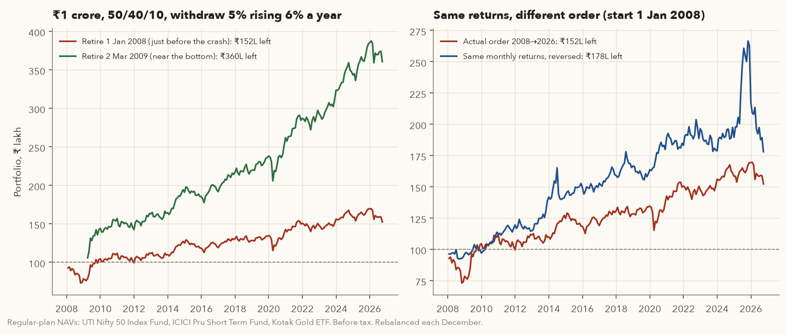
While you are saving, the order of good and bad years does not change your final CAGR. Once you are withdrawing, it does: a crash early in retirement forces you to sell more units at low prices, and those units are not there for the recovery. This is sequence-of-returns risk, the "sequence risk" of Varsity's asset-allocation chapter.
Two retirees, 14 months apart
- Plan: withdraw 5% of the starting corpus in year 1 (₹41,667 a month), raised 6% each year for inflation; rebalance to 50/40/10 each December.
- Retiree A starts on 1 Jan 2008, just before the global financial crisis. A 50/40/10 mix of these funds lost 22.4% in 2008, and after withdrawals the portfolio was down to ₹72.9 lakh by 31 Oct 2008. By 30 Sep 2026 A has withdrawn ₹1.65 crore and has ₹1.52 crore left; the monthly withdrawal has grown to ₹1,18,931.
- Retiree B starts on 2 Mar 2009, near the bottom. By 30 Sep 2026 B has withdrawn ₹1.49 crore and has ₹3.60 crore left.
- Same returns, reversed order (A's monthly returns from 2026 back to 2008): ₹1.78 crore left, after the same ₹1.65 crore of withdrawals.
How long did different withdrawal rates last? For retirements starting each January from 2008 to 2012, here is what was left after 14 years, deflated at 6% a year to the starting year's money (₹1 crore = 100 lakh at the start):
| Start → after 14 years (real ₹ lakh) | 3% a year | 4% | 5% | 6% |
|---|---|---|---|---|
| Jan 2008 | 105.3 | 85.9 | 66.6 | 47.2 |
| Jan 2009 | 149.8 | 131.3 | 112.8 | 94.3 |
| Jan 2010 | 111.6 | 92.4 | 73.3 | 54.1 |
| Jan 2011 | 107.2 | 88.1 | 68.9 | 49.8 |
| Jan 2012 | 142.6 | 122.4 | 102.3 | 82.1 |
The "4% rule" (withdraw 4% of the starting corpus, raise it with inflation, and the money lasts 30 years) comes from US data with lower inflation. Our Indian windows are only 14–18 years long, start from just a few dates, ignore tax and use regular-plan NAVs. At 5–6% withdrawals with 6% inflation, real wealth shrank in most windows: fine for 14 years, worrying for a 30-year retirement. Use a lower rate (3–4%), keep flexibility to cut spending after bad years, and review annually.
The bucket strategy for retirement
A common way to manage sequence risk is three buckets: bucket 1 holds 1–2 years of withdrawals in liquid or money-market funds (the SWP comes from here); bucket 2 holds the next 3–5 years in short-duration debt or a conservative hybrid / BAF; bucket 3 holds the rest in equity for growth. Refill bucket 1 from bucket 3 after good equity years and from bucket 2 after bad ones, so you are never forced to sell equity in a crash. It is rebalancing with a timetable, and the tax playbook of part 14 applies to every refill.
19. In your framework, and try it yourself
framework.funds implements the tools of chapters 14–16: load_nav(code) and search_schemes(query) for AMFI NAVs (cached under data/mf/); xirr, cagr, rolling_returns and sip_simulate(..., step_up_pct=10); fund_tax_class, fund_capital_gains (FIFO, lot by lot) and harvest_plan; and rebalance_backtest(prices, weights, method='none'|'calendar'|'band', ...) with lot-level tax, costs, monthly SIPs and sip_to_underweight=True for cash-flow rebalancing. All fund tax rates live in framework/config.py with sources and an as-of date. From the command line: .venv/bin/python -m framework.funds rebalance --help. The framework's backtest is a separate implementation, so its numbers differ slightly from this chapter's script: it does not carry losses forward between years; its band is a plain ± band in percentage points for every asset (0.05 means ±5 points even for 10% gold), not the 5/25 rule; and trading costs are zero unless you pass costs_bps. The chapter's script is course/scripts/ch16_figures.py.
All snippets read files from the course repository's data/ folder. Save each as a .py file and run it from the repository's root folder with .venv/bin/python snippet.py. Snippets 1–3 need only pandas (snippet 2 needs nothing).
1. Return, risk and correlation of the asset classes (reproduces the table in part 3):
import numpy as np
import pandas as pd

nav = pd.read_csv("data/extra/ch16_navs.csv", index_col=0, parse_dates=True)
nav = nav.loc["2013-01-02":"2026-09-30"]
days = pd.bdate_range(nav.index[0], nav.index[-1])
nav = nav.reindex(nav.index.union(days)).ffill().reindex(days)   # same calendar for all

for col in ["NIFTY50", "MIDCAP", "NASDAQ100", "GILT", "SHORTDEBT", "LIQUID", "GOLD"]:
    s = nav[col].dropna()
    years = (s.index[-1] - s.index[0]).days / 365.25
    cagr = (s.iloc[-1] / s.iloc[0]) ** (1 / years) - 1
    m = pd.concat([s.iloc[:1], s.resample("ME").last()])
    vol = m.pct_change().std() * np.sqrt(12)
    mdd = (s / s.cummax() - 1).min()
    print(f"{col:10s} CAGR {cagr:6.1%}  vol {vol:5.1%}  max drawdown {mdd:6.1%}")

monthly = nav.drop(columns="SMALLCAP").resample("ME").last().pct_change().dropna()
print(monthly.corr().round(2))
# NIFTY50 CAGR 11.1%, vol 15.7%, max drawdown -38.4% ... GOLD 11.0%, 15.4%, -25.5%; corr Nifty-gold -0.11
2. A goal calculator (future cost, level SIP, step-up SIP):
def sip_needed(target, annual_return, months):
    i = (1 + annual_return) ** (1 / 12) - 1
    return target * i / (((1 + i) ** months - 1) * (1 + i))     # paid at the start of each month

def stepup_fv(first_sip, annual_return, years, step):
    i = (1 + annual_return) ** (1 / 12) - 1
    total, amt = 0.0, first_sip
    for y in range(years):
        for m in range(12):
            total += amt * (1 + i) ** ((years - y) * 12 - m)
        amt *= 1 + step
    return total

goal = 20_00_000 * 1.08 ** 12                    # Rs 20 lakh today, 8% inflation, 12 years
print(f"goal Rs {goal:,.0f}")                     # 5,036,340
print(f"level SIP at 8.55%: Rs {sip_needed(goal, 0.0855, 144):,.0f}")          # 20,469
print(f"10% step-up, first SIP: Rs {goal / stepup_fv(1, 0.0855, 12, 0.10):,.0f}")  # 12,597
The step-up figure from this snippet uses a constant 8.55%, so it is lower than the ₹13,352 of part 7, which used the glide path's falling returns.
3. A rebalancing ticket for your own holdings (drift, band check and the trades; replace the values with yours):
target = {"equity": 0.60, "debt": 0.30, "gold": 0.10}
values = {"equity": 17_96_436, "debt": 9_55_400, "gold": 6_02_204}   # Rs, from your statement
next_sips = 6 * 25_000                                                # new money you will add soon

total = sum(values.values())
for a in target:
    w = values[a] / total
    band = min(0.05, 0.25 * target[a])
    flag = "OUTSIDE band" if abs(w - target[a]) > band else "ok"
    print(f"{a:7s} {w:6.1%} (target {target[a]:.0%}, band +/-{band:.1%}) {flag}")

# full rebalance today
for a in target:
    print(f"full rebalance: {a:7s} trade Rs {target[a] * total - values[a]:+,.0f}")
# tax-smarter: new money to the most underweight asset first, then trim only what is still outside its band
after = dict(values)
after["equity"] += next_sips
tot2 = sum(after.values())
trim_gold = max(after["gold"] - 0.125 * tot2, 0)
print(f"sell gold Rs {trim_gold:,.0f} (vs Rs {values['gold'] - 0.10 * total:,.0f} for a full rebalance)")
# sell gold Rs 164,199 (vs Rs 266,800 for a full rebalance)
4. The framework's lot-level rebalancing backtest:
import sys; sys.path.insert(0, ".")                 # run from the repository root
import pandas as pd
from framework.funds import rebalance_backtest

px = pd.read_csv("data/extra/ch16_navs.csv", index_col=0, parse_dates=True)
px = px.loc["2013-01-02":, ["NIFTY50", "SHORTDEBT", "GOLD"]]
classes = {"NIFTY50": "equity_oriented", "SHORTDEBT": "specified_debt", "GOLD": "other"}
for method in ["none", "calendar", "band"]:
    res = rebalance_backtest(px, {"NIFTY50": 0.6, "SHORTDEBT": 0.3, "GOLD": 0.1}, method=method,
                             freq="YE", band=0.05, tax_classes=classes, listed={"GOLD": True},
                             slab_rate=0.30, initial=1_000_000, monthly_sip=20_000)
    m = res["metrics"]
    print(f"{method:9s} CAGR {m['cagr']:.2%}  vol {m['vol']:.1%}  maxDD {m['max_drawdown']:.1%}  "
          f"tax paid Rs {m['tax_paid']:,.0f}  after exit tax Rs {m['post_tax_value']:,.0f}")
# none: CAGR 10.50% ... after exit tax Rs 10,261,184; band: CAGR 10.89% ... Rs 10,730,292
These figures differ a little from the table in part 13 (bands: ₹1,07,30,292 against ₹1,06,36,972 after exit tax; never rebalance: ₹1,02,61,184 against ₹1,02,57,467). The framework uses a flat ±5-point band for every asset, where the table uses 5 points or 25% of the target, whichever is tighter (±2.5 points for gold), and it measures volatility on a time-weighted index. The methods come out in the same order.
Exercise: add sip_to_underweight=True to the "none" run to test cash-flow rebalancing, change the slab to 0.20, or swap "GOLD" for "NASDAQ100" and watch what rebalancing does to a trending asset. To rebuild every number in this chapter, run course/scripts/ch16_data.py --refresh (downloads NAVs) and then course/scripts/ch16_figures.py.
20. Practical checklist
- Term and health insurance in place; emergency fund of 3–12 months' expenses in savings plus a liquid fund, outside the allocation.
- Every goal written down with amount (today's money), inflation, date and its own allocation.
- EPF, PPF, FDs and gold jewellery counted in the debt and gold totals.
- Strategic allocation chosen from risk capacity, tolerance and need, whichever is lowest, and written into an IPS.
- One fund or ETF per asset class; direct plans; tax class, TER and tracking checked (chapter 14).
- Glide path written for each goal with a date; money for goals under 3 years away out of equity.
- Bands set (5 points or 25% of target, whichever is tighter); checked quarterly.
- New money directed to the underweight asset before any sale.
- Before any sale: exit load, 12/24-month dates of the oldest lots, this year's LTCG used so far, available losses.
- February–March: equity LTCG harvested up to ₹1.25 lakh; any rebalancing sales sized to the exemption; buy back the next trading day.
- Family asset location considered; clubbing rules respected; a CA consulted for gifts or large moves.
- ETF premium to iNAV checked before buying international or thin ETFs.
- April: SIP step-up; IPS reviewed; after 1 February each year, tax rules re-checked and
framework/config.pyupdated. - In retirement: 1–2 years of withdrawals in a liquid bucket; SWP rather than IDCW; withdrawal rate reviewed yearly.
21. Key takeaways
- Asset allocation (the split between equity, debt, gold and others) explains most of a portfolio's ups and downs. Get it right before choosing funds.
- 2013–2026 in India: Nifty 50 fund 11.1% a year with a −38.4% worst fall; short-term debt 8.4% with −3.4%; gold 11.0% with −25.5% and a six-year flat spell; Nasdaq 100 24.3% in rupees, a decade that may not repeat.
- Mid and small caps fell as hard as large caps in every crash. Gold and short-term debt cushioned all four falls since 2020; international equity helped in only two.
- The emergency fund comes first and stays outside the allocation. Goals under 3 years away do not belong in equity.
- Plan goals with FV = PV × (1+π)ⁿ and the SIP formula, use conservative returns, add a step-up, and glide to debt as the date nears. SEBI's new Life Cycle Funds do the glide for you.
- A P/E-based tactical rule beat a static 60/40 by 0.21 points a year since 2021, with four times the trading and before tax: too little to rely on.
- Rebalancing is mainly risk control. In 2013–2026 it cut volatility from 10.3% to about 9.4% and added a little return; with a trending asset (Nasdaq 100) it cost two points a year. The chosen month alone moved the result by 5%.
- After tax, rebalancing taxes were small next to the exit tax every method carries. The tax-aware method (new money first, sales inside the ₹1.25 lakh exemption, long-term lots, yearly harvesting) ended about ₹6 lakh ahead of never rebalancing on ₹42.8 lakh invested, but most of that lead came from rebalancing in a lucky month; the reliable part, yearly harvesting, was worth about ₹1 lakh.
- Hybrid funds rebalance without creating tax for you, but check their real drawdowns, costs and tax class.
- In retirement, use SWPs (only the gain part is taxed), a liquid bucket for 1–2 years of spending, and a cautious withdrawal rate: the order of returns matters as much as their average.
22. Quiz and exercises
Q1. Your portfolio is ₹10 lakh: ₹6.5 lakh equity, ₹2.7 lakh debt, ₹0.8 lakh gold. Target 60/30/10 with 5/25 bands. Which assets are outside their bands, and what trades restore the target?
Weights: equity 65%, debt 27%, gold 8%. Bands: equity 55–65% (min(5, 25% × 60 = 15) = 5 points), debt 25–35% (min(5, 7.5) = 5), gold 7.5–12.5% (min(5, 2.5) = 2.5). Equity is exactly at its upper edge, debt and gold are inside, so nothing is outside; a strict band rule does nothing. If you rebalanced anyway: Trade = target × V − Vi: equity 6,00,000 − 6,50,000 = sell ₹50,000; debt 3,00,000 − 2,70,000 = buy ₹30,000; gold 1,00,000 − 80,000 = buy ₹20,000. Better: send the next SIPs to debt and gold.
Q2. Using the measured volatilities (Nifty 15.75%, gold 15.36%) and correlation −0.11, what is the volatility of an 80/20 Nifty/gold portfolio?
\( 0.8^2 \times 0.1575^2 = 0.64 \times 0.024806 = 0.015876 \). \( 0.2^2 \times 0.1536^2 = 0.04 \times 0.023593 = 0.000944 \). Cross term \( 2 \times 0.8 \times 0.2 \times (-0.11) \times 0.1575 \times 0.1536 = -0.000851 \). Sum = 0.015969; \( \sigma_p = \sqrt{0.015969} = \mathbf{12.64\%} \), against a weighted average of 15.67%. Two assets about as volatile as each other, combined, are much less volatile than either.
Q3. A goal costs ₹10 lakh today, is 8 years away, and its inflation is 7%. What is the future cost, and what level monthly SIP (paid at the start of each month) reaches it at 9% a year?
FV = 10,00,000 × 1.078 = 10,00,000 × 1.71819 = ₹17,18,186. i = 1.091/12 − 1 = 0.7207%. (1 + i)96 = 1.098 = 1.99256. SIP = 17,18,186 × 0.007207 / (0.99256 × 1.007207) = 12,383 / 0.99971 ≈ ₹12,387 a month. With 8 years to go, most of it should not stay in equity until the end: plan a glide path from about year 5.
Q4. Why does Brinson's "93.6%" not mean that 93.6% of your return comes from asset allocation?
The 93.6% (Brinson, Hood and Beebower, 1986) is the share of the variation of one fund's quarterly returns over time explained by its policy mix, which is high mainly because every portfolio moves with the markets it holds. Ibbotson and Kaplan (2000) showed that allocation explains only about 40% of the differences between investors' returns, and about 100% of the return level on average. The practical message is the same: choose the mix carefully and keep costs low.
Q5. Your 60/30/10 portfolio has drifted to 66/26/8. You add ₹30,000 a month. Which rebalancing method should you try first, and why?
Cash-flow rebalancing: direct the SIP to debt and gold until they are back near target. It creates no capital gain, no tax and no exit load. Equity at 66% is just outside its 55–65% band; a few months of SIPs into debt and gold will bring it back. Sell only if new money cannot close the gap within a reasonable time (say, two quarters), and then do it in February–March using the ₹1.25 lakh exemption.
Q6. In March you need to sell ₹2 lakh of an equity index fund to rebalance. You have already booked ₹80,000 of long-term gains on shares this tax year. The fund's oldest lots have a gain share of 40%. What is the tax, and how could you reduce it?
Gain on the sale = 40% × 2,00,000 = ₹80,000 (long-term, assuming the oldest lots are over 12 months). Total LTCG this year = 80,000 + 80,000 = ₹1,60,000. Taxable = 1,60,000 − 1,25,000 = ₹35,000. Tax = 35,000 × 12.5% × 1.04 = ₹4,550. To reduce it: sell only ₹1,12,500 now (gain ₹45,000, which uses exactly the remaining exemption) and the rest in April, in the new tax year with a fresh exemption; or direct new money instead; or offset with any capital loss you can book.
Q7. You hold gold through a gold ETF bought 13 months ago and a gold FoF bought 13 months ago, each with a ₹50,000 gain. You are in the 30% slab. What is the tax on selling each?
Gold ETF (listed): long-term after 12 months, so 50,000 × 12.5% × 1.04 = ₹6,500. Gold FoF (unlisted units, not equity-oriented): long-term only after 24 months, so this gain is short-term at slab: 50,000 × 30% × 1.04 = ₹15,600. Waiting 11 more months for the FoF would cut the tax to ₹6,500, if the plan allows.
Q8. You gift ₹5 lakh to your non-working spouse, who invests it in a debt fund that gains ₹40,000. You also gift ₹5 lakh to your retired mother (pension ₹5 lakh, no other income), who buys the same fund and gains ₹40,000. Who pays tax on each gain?
Spouse: the clubbing rule (s.99 of the new Act, old s.64) adds income from assets gifted to a spouse to your income: ₹40,000 at your 30% slab = ₹12,480 with cess. Mother: no clubbing for gifts to parents; the gift itself is tax-free (gift from a relative). Her ₹40,000 gain is slab income; her total income ₹5.4 lakh is under ₹12 lakh, so the rebate makes her tax ₹0. (Confirm the details with a CA.)
Q9. In this chapter's lump-sum backtest, annual rebalancing in March ended at ₹41.89 lakh and in December at ₹39.80 lakh, before tax. What does this tell you, and what would you do about it?
The ₹2.09 lakh (about 5%) gap comes only from which day of the year the rule happened to trade on: "timing luck". It means small differences between rebalancing methods in one backtest are not evidence that one method is better. Practical responses: use bands (trade when drift is large, not on a date), or rebalance in smaller steps (for example half the drift each quarter), and choose the month for tax reasons (February–March, inside the exemption), not because it "won" a backtest.
Q10. Why did rebalancing cost two points a year in the 50/30/20 Nifty/Nasdaq 100/debt portfolio, and does that mean you should not rebalance?
The Nasdaq 100 rose 24.3% a year in rupees, far ahead of the Nifty, almost without a break. Rebalancing kept selling it to buy the laggards, so the portfolio held less of the winner: 15.0% a year against 17.0% (₹60.41 lakh against ₹77.52 lakh after tax). It still lowered volatility (11.7% → 10.4%). It does not mean "never rebalance": without rebalancing, the Nasdaq share would have grown far beyond the 30% you chose, and your portfolio's fate would depend on one market. Rebalancing is insurance against concentration; this was a decade in which the insurance was not needed.
Q11. A retiree needs ₹3 lakh a year. Option 1: hold an equity-oriented fund and take an SWP whose gain share is 50%. Option 2: take the same ₹3 lakh as IDCW. The retiree's slab is 20% and no other LTCG is booked. Compare the tax.
SWP: gain = 50% × 3,00,000 = ₹1,50,000 long-term (if units are over 12 months old). Taxable = 1,50,000 − 1,25,000 = ₹25,000; tax = 25,000 × 12.5% × 1.04 = ₹3,250. IDCW: the full ₹3,00,000 is income at 20% slab: 3,00,000 × 20% × 1.04 = ₹62,400 (ignoring the rebate, which depends on total income). The SWP returns your own capital tax-free and taxes only the gain, at a lower rate.
Q12. Exercise: run snippet 1 with the window 2015-01-01 to 2026-09-30. Which asset's CAGR changes most compared with the 2013 start, and why?
Run it and compare. Expect gold to change a lot: it fell in 2013 and 2014, so starting in 2015 skips two losing years and raises its CAGR, while equity starts after its strong 2014 and its CAGR falls slightly. The lesson: long-run statistics depend on the start and end dates, especially for assets with long flat or falling spells. Always check several windows (rolling returns, chapter 14).
Q13. Exercise: write your own IPS from the template in part 17, then use snippet 3 with your real holdings. Is any asset outside its band today? If yes, how much of the gap can the next six months of SIPs close?
There is no single answer. Check your work: weights sum to 100%; bands use min(5 points, 25% × target); the tax-smarter plan sends new money to the most underweight asset first and sells only what is still outside the band, choosing lots that are long-term and, for equity, gains inside the remaining ₹1.25 lakh exemption.
23. Sources
Zerodha Varsity, Module 11, Personal Finance – Mutual Funds (concepts; explained here in our own words, with figures updated where Varsity's are older; for example Varsity's review chapter still mentions the ₹1 lakh exemption and debt-fund indexation, both since replaced): 2. Personal Finance Math (Part 1) · 3. Personal Finance Math (Part 2) · 4. The Retirement Problem (Part 1) · 5. The Retirement Problem (Part 2) · 26. The Mutual Fund Portfolio · 28. Asset Allocation, An Introduction · 29. Exchange-traded Funds (ETF) · 31. Personal Finance Review (Part 1) · 32. Personal Finance Review (Part 2). Module 9, Risk Management & Trading Psychology: Risk (Part 2) – Variance & Covariance · Risk (Part 4) – Correlation Matrix & Portfolio Variance · Expected Returns · Portfolio Optimization (Part 1).
Law and regulation (checked 2 Oct 2026): Income-tax Act, 2025 as amended by the Finance Act, 2026 (text): s.2(101) short-term capital asset (12/24 months), s.76 specified mutual fund (old 50AA), s.92(2)(m) and (3) gifts (old 56(2)(x)), s.99 clubbing (old 64), s.108–111 set-off and carry-forward (old 70–74), s.196 STCG (old 111A), s.197 LTCG (old 112), s.198 LTCG on equity and equity-oriented fund definition (old 112A) · ClearTax: old vs new section mapping · Outlook Money: MF tax reckoner 2026-27 (no change to fund capital-gains rates in Budget 2026) · AMFI: tax regime for mutual funds · ClearTax: SGB capital gains from 1 Apr 2026 (exemption only for original subscribers held to maturity) · SEBI circular HO/24/13/15(2)2026-IMD-RAC4/I/5764/2026, 26 Feb 2026: Categorization and Rationalization of Mutual Fund Schemes (hybrid ranges, Life Cycle Funds, end of solution-oriented schemes) · PPF 7.1% for Oct–Dec 2026 · EPF 8.25% for 2025-26 · ICICI Pru Short Term Fund: exit load nil · UTI Nifty 50 Index Fund: exit load nil.
Research: Brinson, G., Hood, L. R. and Beebower, G. (1986), "Determinants of Portfolio Performance", Financial Analysts Journal 42(4) · Ibbotson, R. and Kaplan, P. (2000), "Does Asset Allocation Policy Explain 40, 90, or 100 Percent of Performance?", Financial Analysts Journal 56(1).
Data: daily NAVs from AMFI via mfapi.in (UTI Nifty 50 Index Fund Direct 120716; Motilal Oswal Nifty Midcap 100 ETF 114456; Motilal Oswal Nifty Smallcap 250 Index Fund Direct 147623; Motilal Oswal Nasdaq 100 ETF 114984, split-adjusted; HDFC Gilt Fund Direct 119116; ICICI Prudential Short Term Fund Direct 120754; SBI Liquid Fund Direct 119800; HDFC Balanced Advantage 118968, ICICI Pru Balanced Advantage 120377, ICICI Pru Multi-Asset 120334, SBI Multi Asset Allocation 119843 (direct); regular plans UTI Nifty 50 Index 100822, ICICI Pru Short Term 101758; Kotak Gold ETF 106193; Nippon India Silver ETF 149758), saved in data/extra/ch16_navs.csv, ch16_hybrid_navs.csv, ch16_long_navs.csv and ch16_extras.csv; GOLDBEES, MON100 and EMBASSY prices from NSE via Yahoo Finance (two GOLDBEES bad prints in Dec 2019 removed); Nifty 50 P/E from NSE via craytheon.com (data/extra/ch08_nifty_pe_pb_dy_weekly_craytheon.csv). Downloads: course/scripts/ch16_data.py; all calculations and figures: course/scripts/ch16_figures.py with ch16_lib.py (numbers saved to data/extra/ch16_numbers.json). Examples are historical analysis for education, not recommendations or tax advice.