
Risk Management & Trading Psychology
1. What you'll learn and why it matters
Chapters 2 to 10 were about finding trades and investments. This chapter covers the part that decides whether you are still in the game after five years: how much you bet, how much you can lose, and how you behave while losing. Most traders spend 90% of their effort on entries. Most of the damage comes from the other 10%.
The numbers are stark. SEBI's study of individual traders in equity derivatives for FY25–FY26 found that 87.7% of individual F&O traders made a net loss in FY26, with aggregate net losses of about ₹91,685 crore. Even before transaction costs, 82.1% were losing. Few of those people lacked information or chart patterns. What most lacked was position sizing, a stop they respected, and a process that kept their emotions out of the order window.
By the end of this chapter you will be able to:
- Name the kinds of risk you carry (systematic, company-specific, liquidity, gap, leverage, concentration, correlation) and say which ones diversification removes and which ones it cannot touch.
- Compute variance, covariance, correlation and portfolio volatility by hand and with a correlation matrix built from real NSE data, then trace an efficient frontier, and see why it fails out of sample.
- Estimate a portfolio's one-day Value at Risk three ways and explain why VaR broke down in March 2020.
- Size any trade: fixed amount, percentage margin, the 1–2% risk rule, ATR/volatility sizing, equity-curve sizing, Kelly and half-Kelly, and futures lots.
- Calculate R-multiples, expectancy and break-even win rate, and use Monte Carlo simulation to see your probability of a 30% or 50% drawdown.
- Recognise the biases that wreck traders (loss aversion, disposition effect, overconfidence, confirmation, recency, anchoring, FOMO, revenge trading) and put a written rule against each one.
- Keep a trading journal, run a monthly review, and write your own one-page trading plan.
The chapter has three parts. You don't need to read them in one sitting.
- Part A, portfolio risk (Sections 2–6, about 35 min): diversification, correlation, the efficient frontier and Value at Risk. Most useful for long-term investors building a portfolio. A checkpoint box at the end of Section 6 sums it up.
- Part B, sizing and survival (Sections 7–14, about 45 min): recovery maths, position sizing for shares and futures lots, expectancy, Kelly, drawdowns and portfolio heat. Everyone should read this part, and swing and futures traders should read it twice. A checkpoint box at the end of Section 14 sums it up.
- Part C, behaviour (Sections 15–18, about 25 min): the biases that make people break their own rules, the journal, and your written trading plan.
Short on time? Read Sections 7, 9.2, 10, 11, 13.1 and 14 first, then come back for the rest. The formulas look heavy in places, but every one has a worked example with real numbers right below it.
Swing traders take dozens of trades a year. Over that many trades, bet size matters more than any single entry. Long-term investors face a different risk: concentration and deep drawdowns. Several blue chips in our data fell 50% or more in 2024–26. Futures traders run on 5–9x leverage, so the arithmetic of ruin arrives fast: one bad day can wipe out a quarter of the margin. The tools differ a little for each group. The principle is the same: decide the loss before you decide the trade.
About the data: every number in this chapter comes from course/scripts/ch11_figures.py, which reads the course's daily NSE data (to 30 Sep 2026), the NSE futures bhavcopy and SPAN file for 30 Sep 2026, and the 2,187 completed historical trades from the four swing setups of Chapter 5 (S1 trend pullback, S2 52-week breakout, S3 support bounce, S4 weekly trend + daily trigger, all with R net of costs; R means a trade's profit or loss measured in units of the risk planned at entry, so −1R is a normal stop-out, defined fully in Section 11). All the numbers are saved in data/extra/ch11_results.json.
2. What "risk" means, and the kinds you will face
In everyday language risk means "something bad might happen". In markets it has two working meanings. Keep both in mind:
- Risk as volatility: how widely returns swing around their average. This is what portfolio maths measures (standard deviation, variance, VaR).
- Risk as permanent loss: the chance of losing money you never get back, because you sold at the bottom, a company failed, or leverage forced you out. Traders and investors actually fear this one, and position sizing and stops are built to control it.
2.1 Systematic vs unsystematic risk
Varsity starts the module with this split, and it is the most useful one to learn first.
- Unsystematic (company-specific) risk lives inside one business: a bad quarter, a management exit, a new competitor, a regulatory order against that company. It hits the stock and usually not its peers. Diversification reduces it, because bad news at one company is offset by ordinary days at the others.
- Systematic (market) risk is common to the whole system: interest rates, a global sell-off, war, a pandemic, a tax change on all equities. Every stock is exposed. Diversification cannot remove it. You can only reduce it by holding less equity, holding cash or uncorrelated assets, or hedging with index futures or puts (Chapters 9 and 10).
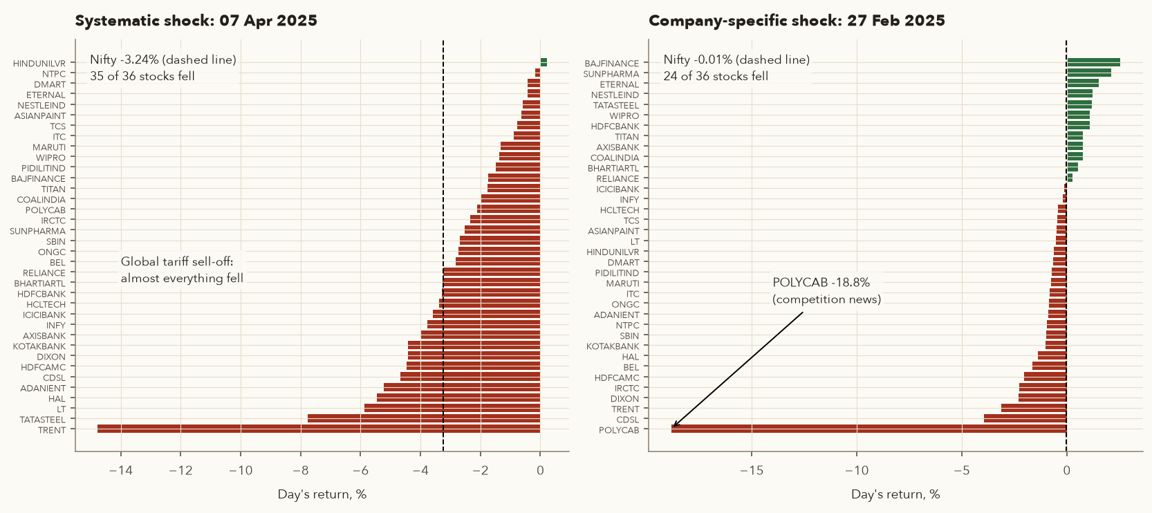
Company-specific risk, measured
- Previous close (25 Feb 2025; 26 Feb was a market holiday): ₹5,765.60. Open on 27 Feb: ₹5,400.00, already a gap of \(5400/5765.6-1 = -6.3\%\).
- Low of the day ₹4,656.00. Close ₹4,679.55. One-day return \(4679.55/5765.6-1=-18.84\%\).
- The same day the Nifty moved −0.01% and the median stock in our list moved −0.57%. The loss was almost entirely company-specific.
- Held as 1 of 15 equal-weight positions (6.67% each), the hit to the portfolio is about \(0.0667\times(-18.84\%) \approx -1.26\%\). As a 30% position it is −5.65%. Position weight is what turns company risk into portfolio risk.
Systematic risk: nowhere to hide inside equities
On 7 Apr 2025 the Nifty fell 3.24%, India VIX jumped 65.6% to 22.79, 35 of 36 stocks fell, and the median stock lost 2.70%. TRENT fell 14.77% (₹5,562.85 to ₹4,740.95), the market sell-off plus the reaction to its own quarterly business update. Holding more Indian stocks would not have helped that day. Lower equity exposure, cash, gold or a hedge would have.
2.2 The other risks a trader actually meets
| Risk | What it is | Real example from our data | Main control |
|---|---|---|---|
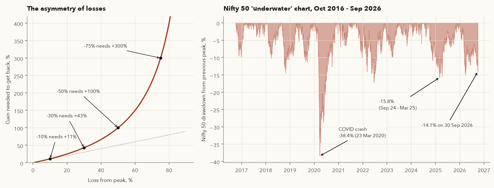
| Market (systematic) | Everything falls together | Nifty −38.4% from 14 Jan to 23 Mar 2020; −15.8% from 26 Sep 2024 to 4 Mar 2025 | Asset allocation, hedges, regime filter (Ch 5), lower size in high VIX |
| Company-specific | One business has a bad event | POLYCAB −18.8% in a day (27 Feb 2025) | Diversification, position limits (e.g. max 10–20% per stock) |
| Gap risk | Price opens beyond your stop, so the stop fills far worse than planned | ONGC opened 6.45% below its previous close on 2 Feb 2026 and stopped a trade out at −3.54R instead of −1R (Section 9) | Smaller size around results/events; options hedge; assume 2–3R worst case |
| Liquidity risk | You cannot exit near the screen price in size | Median daily traded value Jul–Sep 2026: HDFCBANK ₹1,967.8 cr vs IRCTC ₹34.7 cr | Trade liquid names; keep position below ~1% of daily value; use limit orders |
| Leverage risk | Small price moves become large moves on your own money | The Nifty's −3.26% day on 19 Mar 2026 equals about −₹48,000 on one NIFTY futures lot at 30 Sep 2026 prices, 28.8% of its margin in one session (Section 10) | Size by risk not by margin; keep unused margin; never average down a futures loser |
| Concentration risk | Too much money in one stock or theme | An IT-heavy portfolio: TCS −56.5% and INFY −50.7% peak-to-trough (2024–26) | Per-stock and per-sector caps |
| Correlation risk | "Different" positions are really one bet | Five S4 entries on 21 Sep 2026 were all stopped out within 8 days, −5.25R together (Section 14) | Portfolio heat cap, sector limits, count correlated trades as one |
| Model / regime risk | A tested edge stops working | S4 earned +0.30R per trade 2017–2026 overall but −0.10R per trade from 2024 (Section 11) | Monitor live expectancy; equity-curve sizing; small size on new systems |
The table needs one reading habit: most of these risks are invisible on a chart while you are entering. A clean breakout chart doesn't show that it is your fourth bank trade this week, that results are due in two days, or that the stock trades only ₹30 crore a day. Your risk process has to ask those questions for you.
Liquidity differs by a factor of 50 even among large caps
| Stock | Median daily value (₹ crore) | 1% of daily value (₹) |
|---|---|---|
| HDFCBANK | 1,967.8 | 19.68 crore |
| RELIANCE | 1,325.3 | 13.25 crore |
| DIXON | 529.9 | 5.30 crore |
| POLYCAB | 249.4 | 2.49 crore |
| CDSL | 148.9 | 1.49 crore |
| IRCTC | 34.7 | 35 lakh |
A common rule of thumb is to keep an order below about 1% of the stock's typical daily value so that your own order barely moves the price. For a retail account of ₹5–50 lakh every stock above clears that easily. Liquidity risk bites in small caps, on circuit-limit days, and in far-month futures and deep out-of-the-money options. Those are exactly the places beginners drift into.
3. Diversification maths: variance, covariance, correlation
Varsity spends four chapters building portfolio risk from first principles. The logic is simple even though the algebra looks heavy: portfolio risk depends on each stock's own volatility and on how the stocks move together. The "together" part is what diversification works on.
3.1 Variance and standard deviation of one stock
- \(r_t\)
- The stock's return on day \(t\), as a fraction: \(P_t/P_{t-1} - 1\), where \(P\) is the closing price (0.01 = +1%).
- \(n\)
- How many daily returns you have. Six closes give five returns.
- \(\bar r\)
- The mean (average) of those returns. A bar over a symbol always means "average of".
- \(\sum_{t=1}^{n}\)
- "Add up the expression for every day from 1 to \(n\)."
- \(\sigma^2\)
- The variance: the average squared distance of daily returns from their mean. Dividing by \(n-1\) rather than \(n\) is the standard correction for a sample. It makes almost no difference with a year or more of data.
- \(\sigma\)
- The standard deviation (volatility): the square root of the variance, back in "percent per day" units.
- \(\sigma_{\text{daily}},\ \sigma_{\text{annual}}\)
- Volatility per trading day and per year. 252 is roughly the number of trading days in a year.
- Subtract the average return from each day's return, and square the result. Squaring makes every deviation positive and penalises big moves more heavily.
- Add the squares and divide by \(n-1\). That is the variance.
- Take the square root to get the daily standard deviation.
- Multiply by \(\sqrt{252}\) to annualise. This assumes days are roughly independent, so risk grows with the square root of time.
Variance by hand
- Closes 23–30 Sep 2026: 737.25, 728.90, 735.60, 719.05, 722.70, 708.70.
- Daily returns \(r_t = P_t/P_{t-1}-1\): −1.1326%, +0.9192%, −2.2499%, +0.5076%, −1.9372%.
- Mean \(\bar r = -0.7786\%\).
- Squared deviations: 0.00001253, 0.00028824, 0.00021647, 0.00016543, 0.00013424. Sum = 0.00081691.
- Sample variance = 0.00081691 / (5−1) = 0.00020423. Standard deviation = \(\sqrt{0.00020423}=1.429\%\) per day.
Five days is far too few for a real estimate. Varsity suggests at least a year of data, and the rest of this chapter uses two years (1 Oct 2024 to 30 Sep 2026, 495 sessions). The point here is only to see the mechanics.
3.2 Covariance and correlation
- \(A,\ B\)
- Two stocks, for example HDFCBANK and ICICIBANK.
- \(r_{A,t},\ r_{B,t}\)
- The daily return of stock \(A\) and of stock \(B\) on the same day \(t\).
- \(\bar r_A,\ \bar r_B\)
- Each stock's average daily return over the period.
- \(n\)
- The number of days with a return for both stocks.
- \(\text{Cov}(A,B)\)
- The covariance: positive if the two tend to be above (or below) their averages on the same days, negative if one tends to be up when the other is down.
- \(\sigma_A,\ \sigma_B\)
- Each stock's standard deviation, from the formula above.
- \(\rho_{A,B}\)
- The correlation (Greek letter rho): covariance rescaled so it always lies between −1 and +1.
- For each day, multiply stock A's deviation from its average by stock B's deviation from its average. Same-direction days give a positive product, opposite-direction days a negative one.
- Add the products and divide by \(n-1\). That is the covariance.
- Divide by both standard deviations to get the correlation. +1 means lock-step, 0 means no linear relation, −1 means opposite moves.
Covariance asks whether two stocks tend to be above their averages on the same days. The raw number is hard to read, so we scale it into correlation: +1 means they move in lock-step, 0 means no linear relation, −1 means they move in opposite directions. Over the same five days, ICICIBANK's returns gave a covariance with HDFCBANK of −0.0000424 and a correlation of −0.19. Five days of noise, though. Over two years the correlation is +0.51. Always use enough data.
3.3 Two-stock portfolio: where the diversification benefit comes from
- \(\sigma_p^2,\ \sigma_p\)
- The variance and the volatility of the whole portfolio (subscript \(p\)).
- \(w_1,\ w_2\)
- The weights: the share of the money in stock 1 and stock 2, as fractions that add up to 1 (50/50 is 0.5 and 0.5).
- \(\sigma_1,\ \sigma_2\)
- Each stock's own volatility. Use daily or annual figures, but the same for both.
- \(\rho_{12}\)
- The correlation between the two stocks' returns, from the formula above.
How it works: square each weight × volatility and add them. Then add the interaction term, 2 × both weights × correlation × both volatilities. Take the square root of the total for the portfolio's volatility. The lower the correlation, the smaller the interaction term, and the lower the portfolio's risk.
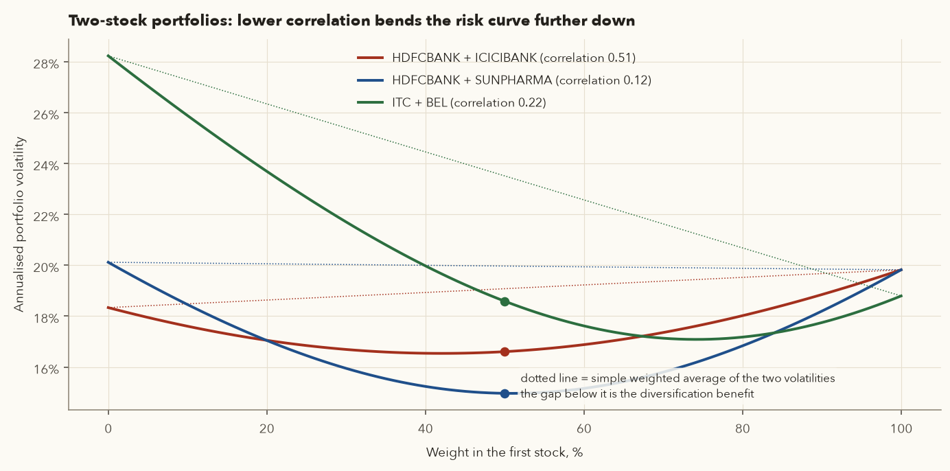
The first two terms are each stock's own risk. The third term is the interaction. If \(\rho=1\), the formula collapses to \(\sigma_p = w_1\sigma_1+w_2\sigma_2\): a plain weighted average, so no benefit at all. Any \(\rho<1\) makes \(\sigma_p\) smaller than the weighted average. That gap is the "free lunch" of diversification.
Plugging real numbers into the formula
- Annual volatilities: HDFCBANK \(\sigma_1=19.82\%\), SUNPHARMA \(\sigma_2=20.12\%\). Correlation \(\rho=0.1235\). Weights 0.5 each.
- \(w_1^2\sigma_1^2 = 0.25\times0.1982^2 = 0.009821\)
- \(w_2^2\sigma_2^2 = 0.25\times0.2012^2 = 0.010120\)
- \(2w_1w_2\rho\sigma_1\sigma_2 = 2\times0.25\times0.1235\times0.1982\times0.2012 = 0.002462\)
- \(\sigma_p^2 = 0.022404\), so \(\sigma_p=\sqrt{0.022404}=14.97\%\).
- Compare: the simple average of the two volatilities is 19.97%. With \(\rho=0\) it would be 14.12%. A low correlation removed about a quarter of the risk without giving up any expected return.
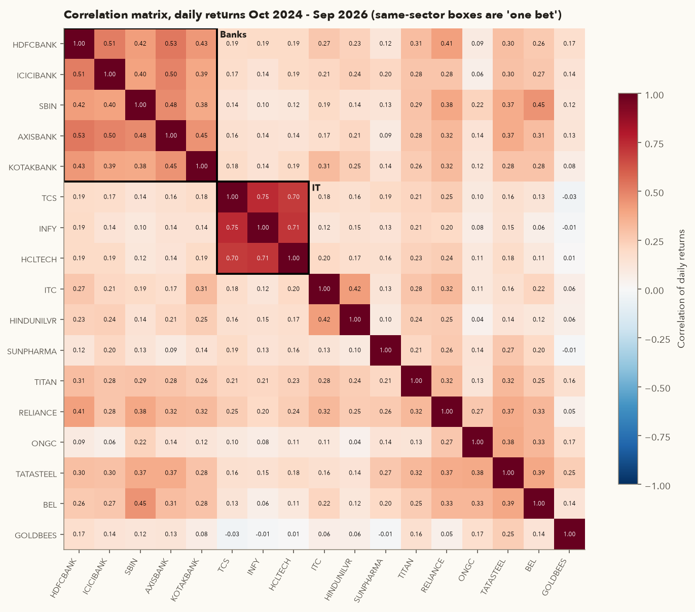
3.4 The correlation matrix: see your hidden bets
With many stocks you need every pairwise correlation. Arranged in a grid, they form the correlation matrix. It is the single most useful risk picture for a swing trader with several open positions, because it shows which "different" trades are really the same trade.
3.5 How many stocks are enough?
If you hold \(n\) equal-weight stocks, portfolio variance is approximately
- \(n\)
- The number of stocks, each holding the same share \(1/n\) of the money.
- \(\sigma_p^2\)
- The portfolio's variance.
- \(\overline{\sigma^2}\)
- The average variance of the individual stocks (the bar means "average").
- \(\overline{\text{Cov}}\)
- The average covariance across every pair of stocks: how much they move together on average.
How it works: the first term is divided by \(n\), so it shrinks as you add stocks: with 10 stocks only a tenth of the average variance is left. The weight on the second term, \(1 - 1/n\), heads towards 1, so the portfolio's variance settles at the average covariance and goes no lower. Take the square root for volatility.
As \(n\) grows, the first term (company-specific risk) shrinks towards zero. The second term (average covariance, the market risk) stays. That is the maths behind "diversification removes unsystematic risk but not systematic risk".
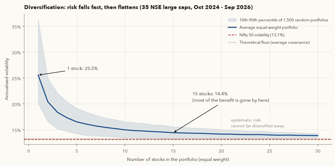
Going from 1 to 10 stocks removes most of the avoidable risk. Beyond 15–20 the extra benefit is tiny, and you begin to own "the index with extra steps". For an investor, 12–20 well-chosen stocks across at least 5–6 unrelated sectors is a sensible range, or simply use an index fund for the core. For a swing trader holding 4–8 positions, the job is to make sure those positions are not all from one correlated block.
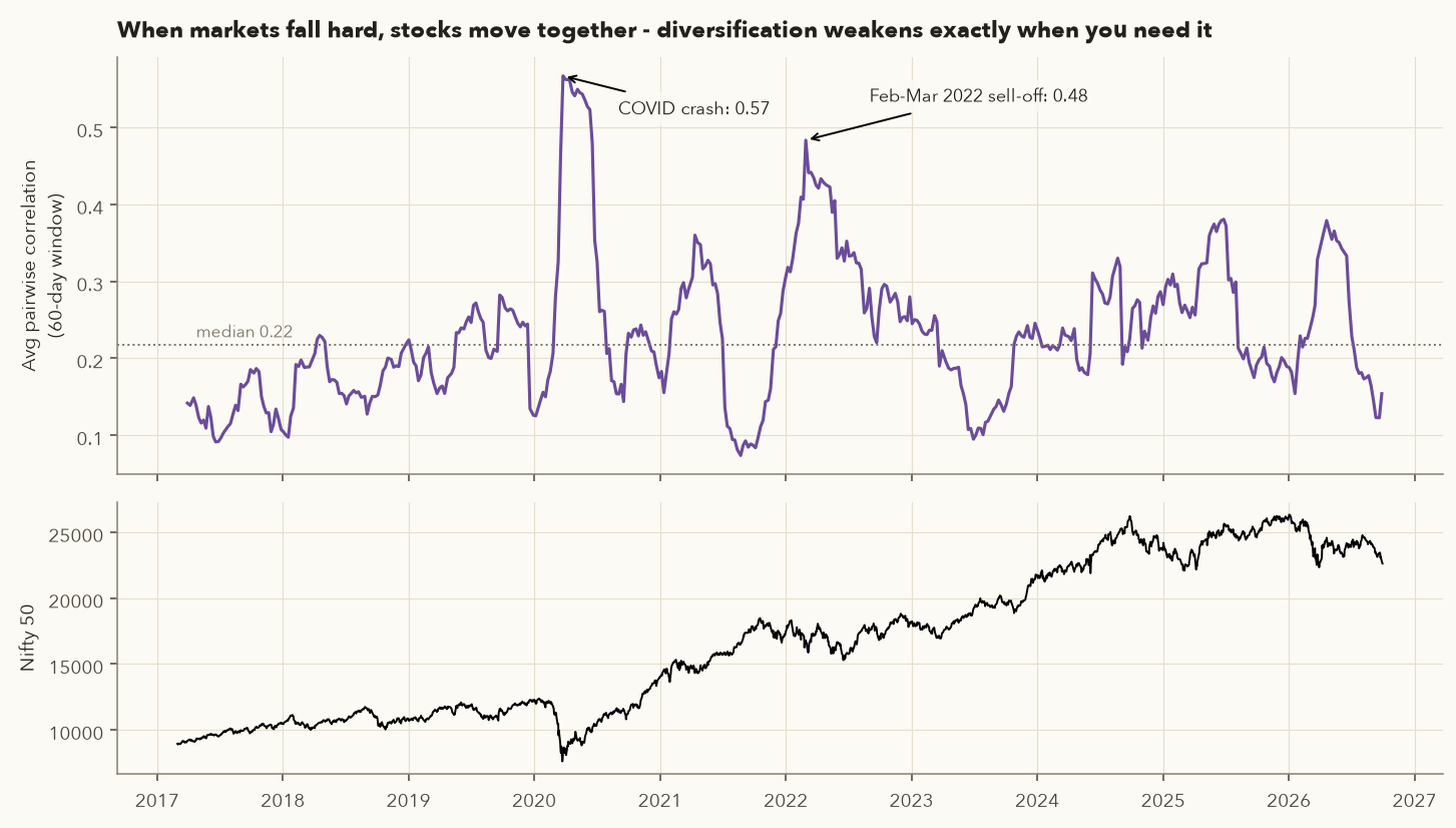
Correlations are measured from the past and they rise in crashes. Section 14 shows the average pairwise correlation of our stocks jumping from a median of 0.22 to 0.57 in March 2020. Diversification is weakest exactly when you need it most. Plan for that.
4. Portfolio variance for many stocks, the equity curve and expected range
Varsity uses matrix algebra to extend the two-stock formula to any number of stocks. The steps are worth knowing once, because Python and Excel then do them for you.
- \(k,\ n\)
- The number of stocks, and the number of trading days of data.
- \(X\)
- An \(n\times k\) table (\(n\) rows of days, \(k\) columns of stocks) of daily excess returns: each stock's return minus its own average return.
- \(X^{\mathsf T}\)
- The transpose of \(X\): the same table turned on its side, so rows become columns. Multiplying \(X^{\mathsf T}X\) adds up "deviation × deviation" for every pair of stocks at once.
- \(\Sigma\)
- The \(k\times k\) variance-covariance matrix: each stock's variance on the diagonal and each pair's covariance off it. (Same Greek letter as the "add up" sign, but standing on its own it names this matrix.) Varsity divides by \(n\), not \(n-1\). With hundreds of days the difference is negligible.
- \(C\)
- The \(k\times k\) correlation matrix (Section 3.4).
- \(w\)
- The list (vector) of portfolio weights, one per stock, adding up to 1.
- \(\sigma\)
- The list of each stock's daily standard deviation.
- \(w\circ\sigma\)
- The \(\circ\) means multiply item by item, so this is the list of "weight × standard deviation" for each stock.
- \(\sigma_p^2\)
- The portfolio's daily variance. Its square root is the daily portfolio volatility.
- Build \(X\): subtract each stock's average return from its daily returns.
- Compute \(\Sigma = X^{\mathsf T}X / n\).
- Divide each entry by the two stocks' standard deviations to get \(C\).
- Multiply the weight × SD list by \(C\), and then by the list again. That gives one number, the portfolio variance. (\(w^{\mathsf T}\Sigma\, w\) is the same calculation done straight from \(\Sigma\).)
- Take the square root for daily volatility, and multiply by \(\sqrt{252}\) for annual. It is the two-stock formula of Section 3.3 extended to every pair. Python, or Excel's
MMULT, does the multiplying for you.
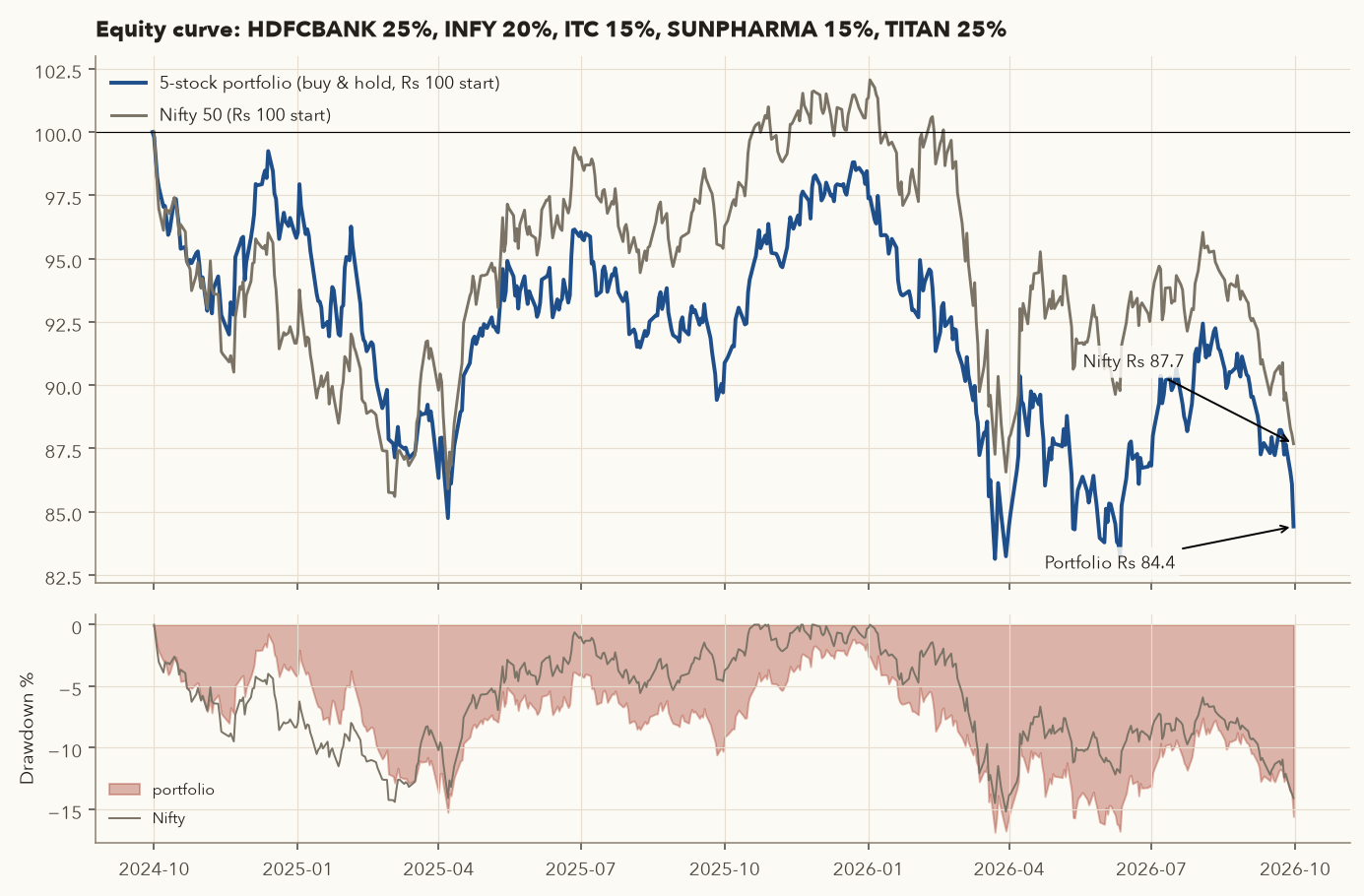
HDFCBANK 25%, INFY 20%, ITC 15%, SUNPHARMA 15%, TITAN 25%
| Stock | Weight | Daily SD | Weight × SD | Mean daily return | Annualised (×252) |
|---|---|---|---|---|---|
| HDFCBANK | 25% | 1.247% | 0.3118% | −0.0308% | −7.76% |
| INFY | 20% | 1.764% | 0.3528% | −0.1001% | −25.23% |
| ITC | 15% | 1.183% | 0.1774% | −0.1040% | −26.20% |
| SUNPHARMA | 15% | 1.266% | 0.1899% | −0.0035% | −0.88% |
| TITAN | 25% | 1.429% | 0.3571% | +0.0445% | +11.20% |
- Pairwise correlations range from 0.118 (INFY–ITC) to 0.307 (HDFCBANK–TITAN), all low.
- \((w\circ\sigma)^{\mathsf T} C (w\circ\sigma) = 0.00007283\) (daily variance). Square root: 0.853% per day.
- Annualised: \(0.853\%\times\sqrt{252}=13.55\%\). The weighted average of the five annual volatilities is 22.05%, so correlation below 1 cut the risk by about 39%.
- Check: computing the SD of the actual daily portfolio returns gives the same 0.853%. The matrix route is just a shortcut.
4.1 The equity curve
Varsity's chapter 6 normalises the portfolio to ₹100 at the start and tracks its value each day. This equity curve is the honest summary of an investment or a trading system: return, path and drawdowns in one picture. Always plot it against a benchmark.
4.2 Expected return and a realistic range
- \(E[R_p]\)
- The expected annual return of the portfolio, as a %. \(E[\ldots]\) means "expected value", i.e. the average outcome.
- \(w_i\)
- The weight of stock \(i\) (its share of the money, as a fraction).
- \(\bar r_i\)
- Stock \(i\)'s average daily return over the data period.
- 252
- Trading days in a year: it turns an average daily return into an annual one.
- \(\sum_i\)
- "Add up over every stock \(i\) in the portfolio."
- \(\sigma_{p,\text{annual}}\)
- The portfolio's annual volatility, from the matrix formula above.
- \(k\)
- How many standard deviations wide the range is. 1 covers about 68% of years if returns were normal, 2 about 95%, 3 about 99.7%.
- Multiply each stock's average daily return by its weight, add them up, and multiply by 252. That is the centre of the range.
- Add and subtract \(k\) times the portfolio's annual volatility to get the range for that confidence level.
What the last two years "predict"
- Weighted annual contributions: HDFCBANK −1.939%, INFY −5.046%, ITC −3.930%, SUNPHARMA −0.132%, TITAN +2.801%. Sum \(E[R_p] = -8.25\%\).
- \(\sigma_p = 13.55\%\). One-SD range: −21.79% to +5.30%. Two-SD: −35.34% to +18.85%. Three-SD: −48.89% to +32.39%.
- The realised buy-and-hold CAGR was −8.29%, consistent, since we measured on the same period.
Read this carefully. The "expected" return is simply the past average projected forward. Two years earlier (Oct 2022 – Sep 2024) the same five stocks averaged +13% to +39% a year each. Means estimated from a couple of years of data are extremely noisy. Volatility and correlation estimates are far more stable than return estimates, so use this method to judge the width of the range, not its centre.
5. Portfolio optimisation and the efficient frontier, and its limits
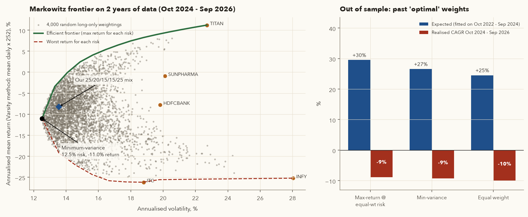
Harry Markowitz's insight, which Varsity's chapters 8–9 walk through with Excel Solver: for any set of stocks you can try every combination of weights and plot each portfolio's risk against its expected return. Two special portfolios stand out:
- the minimum-variance portfolio, the weights that give the lowest possible volatility;
- the efficient frontier, the upper edge of the cloud: for each level of risk, the highest expected return available. Any portfolio below the frontier is "inefficient": another mix gives more return for the same risk.
- \(\min_{w}\)
- "Find the weights \(w\) that make the next expression as small as possible."
- \(w^{\mathsf T}\Sigma w\)
- The portfolio's variance, from the matrix formula in Section 4.
- s.t.
- "Subject to": the rules the weights must obey.
- \(\sum w_i = 1\)
- The weights add up to 100%: all the money is invested.
- \(w_i \ge 0\)
- No weight is negative, so no short selling.
- \(\mu\)
- The list of each stock's expected (average past) return. \(w^{\mathsf T}\mu\) is the portfolio's expected return.
- target return
- The return you ask the portfolio to deliver. Drop this rule and you get the minimum-variance portfolio.
How it works: for one chosen target return, a solver (Excel Solver or Python) tries weights until it finds the mix with the lowest risk. Repeat for many targets and plot each answer's risk against its return: the line traced is the efficient frontier.
Why the frontier is a teaching tool, not a crystal ball
- Fit on Oct 2022 – Sep 2024: annual mean returns were HDFCBANK +13.4%, INFY +20.1%, ITC +28.2%, SUNPHARMA +38.9%, TITAN +22.1%. The "max-return at equal-weight risk" mix put 42.1% in SUNPHARMA and expected +29.5% a year.
- Hold for Oct 2024 – Sep 2026: that mix actually returned −8.91% a year (max drawdown −17.5%). Minimum-variance returned −9.25% and equal weight −10.09%.
- The volatility forecasts held up well: minimum-variance expected 11.18% volatility and realised 12.60%. The return forecasts were useless.
Lesson: optimisers treat noisy past returns as facts and pile into whatever did best recently. Use the frontier's risk insight (combine low-correlation assets, avoid concentration) and treat its return outputs with deep suspicion. Equal weight or simple caps per stock and sector are hard to beat in practice.
6. Value at Risk: historical, variance-covariance and expected shortfall
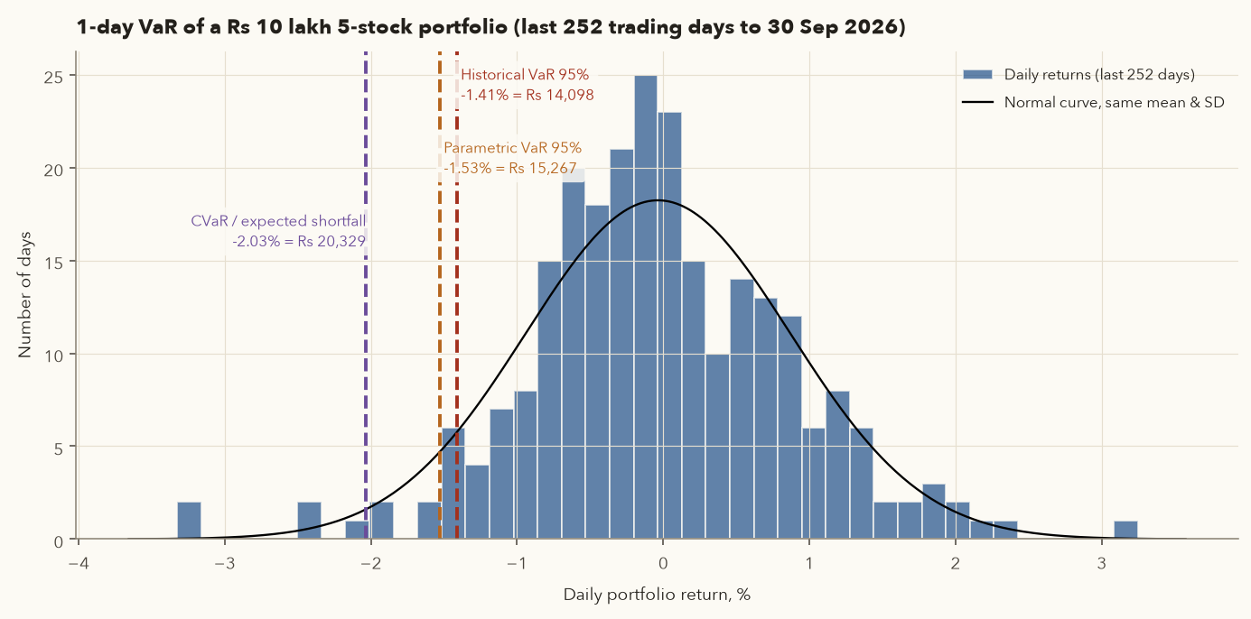
Value at Risk (VaR) answers one question: "On a normal bad day, how much could this portfolio lose?" Formally, the 95% one-day VaR is the loss that should be exceeded on only 5% of days (about one day in twenty, or 12–13 days a year).
- \(\text{VaR}_{95},\ \text{VaR}_{99}\)
- One-day Value at Risk at 95% and 99% confidence, as a % of the portfolio. Written as a positive loss. Multiply by the portfolio value for ₹.
- 5th percentile
- The return that 5% of days were worse than. With 252 days, sort them from worst to best: it sits around the 13th-worst day.
- \(\mu\)
- The portfolio's average daily return (Greek letter mu).
- \(\sigma_p\)
- The portfolio's daily standard deviation (Section 4).
- 1.645, 2.326
- Fixed numbers from the normal (bell) curve: only 5% of outcomes fall more than 1.645 standard deviations below the average, and only 1% more than 2.326 below.
- Expected shortfall (CVaR)
- The average loss on the days that were worse than the VaR cut-off.
- Historical: sort past daily returns and read off the 5th percentile. Flip the sign to report it as a loss.
- Parametric: assume returns follow a bell curve. Take the average return and subtract 1.645 standard deviations (2.326 for 99%). Flip the sign.
- Expected shortfall: average all the returns worse than the 5th percentile. It is always a bigger loss than VaR, because it looks inside the tail rather than at its edge.
A note on vocabulary: Varsity's VaR chapter sorts the portfolio returns and takes the average of the worst 5%. Textbooks call that number expected shortfall or CVaR, and reserve "VaR" for the 5th-percentile cut-off itself. Both are useful. CVaR is always the larger loss, because it averages the tail beyond the cut-off. We compute both below.
One-day VaR three ways
- Historical: sort the 252 daily returns (23 Sep 2025 – 30 Sep 2026). The 5th percentile is −1.41%. 95% VaR = 1.41% × ₹10,00,000 = ₹14,098. The 99% historical VaR is −2.38% = ₹23,814.
- Expected shortfall: the 13 worst days averaged −2.03%, so CVaR95 = ₹20,329. (This is "VaR" the way Varsity computes it.)
- Parametric: mean \(\mu=-0.0359\%\), \(\sigma=0.9063\%\). \(1.645\sigma = 1.4908\%\). VaR95 \(= -(−0.0359\% − 1.4908\%) = 1.53\%\) = ₹15,267. VaR99 = 2.14% = ₹21,439.
- Multi-day: using the square-root-of-time rule, 10-day parametric VaR95 ≈ ₹15,267 × √10 ≈ ₹48,280.
- Back-test: parametric VaR95 was breached on 9 of 252 days versus 12.6 expected. That is reasonable in a calm year. The worst day (23 Mar 2026, −3.32%) was a 3.6-sigma move, which "should" almost never happen under a normal curve. Returns have fat tails: extreme days happen more often than the normal curve predicts (excess kurtosis 1.43; a normal distribution has 0).
6.1 When VaR fails: March 2020
A fair-weather number
- Using all of 2019, the Nifty's daily SD was 0.878% and parametric VaR95 was −1.39%.
- In the crash window of 20 Feb – 30 Apr 2020 (45 sessions), a 5% breach rate would predict about 2.25 breaches. There were 15. In the first half of 2020 there were 23 breaches in 122 days.
- On 23 Mar 2020 the Nifty fell 12.98%: 9.3 times the VaR, a 14.8-sigma event under 2019's normal distribution. On that model it was essentially impossible. It happened anyway.
- A milder repeat: on 7 Apr 2025 the Nifty fell 3.24%, a 3.7-sigma day against the previous year's VaR of −1.43%.
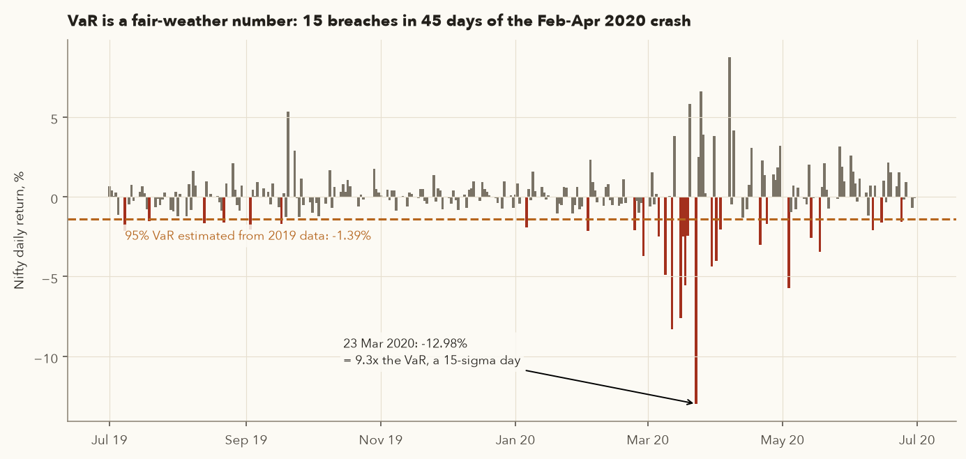
VaR is a good "normal weather" gauge: if your ₹10 lakh portfolio routinely loses ₹15,000 on a bad day and that makes you anxious, you hold too much risk. It says nothing about how bad the worst days are. Always pair it with a stress test: "what if the market does a March 2020 (−13% in a day, −38% peak-to-trough) or an April 2025 (−3% in a day with VIX +66%)?" For a futures trader, a stress test is mandatory. The next sections show why.
- Diversification removes company-specific risk but not market risk. About 10–15 stocks from unrelated sectors gets most of the benefit.
- Correlation is what matters, not the number of names. Two IT stocks (ρ ≈ 0.75) are close to one bet.
- Portfolio volatility comes from weights, volatilities and correlations. Past returns are too noisy to optimise on.
- VaR tells you the size of a normal bad day (about ₹14,000–15,000 on ₹10 lakh for our 5-stock portfolio). It says nothing about crash days.
- Correlations jump in crashes, so always add a stress test: "what if the market falls 13% in a day, or 38% over two months?"
7. Why position sizing comes first: gambler's fallacy and recovery maths
Varsity opens its position-sizing chapters with a poker story: lose the first two small bets, raise the third to "win it back", lose that too, and the buy-in is gone in ten minutes. Two ideas explain why that happens to traders.
7.1 Gambler's fallacy
The gambler's fallacy is the belief that after a run of losses a win is "due". If your trades are roughly independent, the odds on the next trade are the same as they were on the first. A system with a 38% win rate still has a 62% chance of losing the next trade after eight losses in a row. Raising size after losses ("martingale" thinking) leaves your odds unchanged and puts the biggest bets in the worst stretch.
7.2 Recovery maths: losses and gains are not symmetric
- \(L\)
- The loss from the peak, as a positive fraction: a 20% fall is \(L = 0.20\). This fall from a previous high is called a drawdown.
- Gain needed
- The % rise required from the low to get back to the old peak, as a fraction (0.25 = +25%).
How it works: after losing \(L\), you have \(1 - L\) of your money left. To get back to 1 you must multiply it by \(1/(1-L)\). Subtract 1 to express that as a gain. The gain is always bigger than the loss because it is earned on a smaller base.
Example: ₹5,00,000 falls 20% to ₹4,00,000. Gain needed \(= 0.20 / 0.80 = 0.25\), i.e. +25%, since ₹4,00,000 × 1.25 = ₹5,00,000. At \(L = 0.50\) it is \(0.50/0.50 = 1\), i.e. +100%.
| Loss from peak | Gain needed to get back | What it feels like |
|---|---|---|
| −5% | +5.3% | A normal month |
| −10% | +11.1% | Uncomfortable, recoverable |
| −15% | +17.6% | Nifty from Jan 2026 high to 30 Mar 2026 |
| −20% | +25.0% | Most people start breaking rules here |
| −25% | +33.3% | |
| −30% | +42.9% | A year or more of good trading to repair |
| −40% | +66.7% | |
| −50% | +100% | TCS, INFY, IRCTC from their 2024 peaks |
| −60% | +150% | |
| −75% | +300% | Account effectively ruined |
| −90% | +900% |
"Blue chip" does not mean "small drawdown"
| Stock | Peak (date) | Trough (date) | Drawdown | Gain needed | 30 Sep 2026 vs peak |
|---|---|---|---|---|---|
| IRCTC | ₹1,126.0 (22 May 2024) | ₹452.5 (29 Sep 2026) | −59.8% | +148.8% | −59.6% |
| TCS | ₹4,553.8 (30 Aug 2024) | ₹1,982.6 (1 Jul 2026) | −56.5% | +129.7% | −55.0% |
| ADANIENT | ₹3,645.2 (3 Jun 2024) | ₹1,758.8 (30 Mar 2026) | −51.8% | +107.3% | −20.4% |
| INFY | ₹1,999.7 (13 Dec 2024) | ₹985.3 (1 Jul 2026) | −50.7% | +103.0% | −50.3% |
| ITC* | ₹503.4 (26 Sep 2024) | ₹255.5 (31 Aug 2026) | −49.2% | +97.0% | −47.8% |
| DIXON | ₹18,940.2 (17 Dec 2024) | ₹9,673.0 (30 Mar 2026) | −48.9% | +95.8% | −30.8% |
| HDFCBANK | ₹1,012.9 (30 Jul 2025) | ₹687.1 (9 Sep 2026) | −32.2% | +47.4% | −30.0% |
| RELIANCE | ₹1,600.9 (8 Jul 2024) | ₹1,161.9 (4 Mar 2025) | −27.4% | +37.8% | −25.9% |
*In January 2025 ITC demerged its hotels business, and shareholders received ITC Hotels shares separately. In our data, ITC's prices before the demerger are scaled down so the series stays comparable across it. The ITC Hotels shares are not tracked here. Prices are split- and bonus-adjusted (HDFCBANK 1:1 bonus in Aug 2025). The lesson for investors: a concentrated portfolio of "safe" large caps could have sat 50% underwater for two years. Diversification across sectors and a written rule for when a thesis is broken (Chapter 17) are your defence.
Because losses compound against you, the first job of position sizing is to keep drawdowns in the shallow part of the curve, where recovery takes months, not years. Small accounts are tempted to take big bets "to make it worthwhile". Varsity warns against exactly that. A small account blown up teaches you nothing a small account sized properly couldn't.
8. How much capital do you really have? Three equity models
Every sizing rule says "risk X% of your capital". So what is your capital while some of it is already tied up in open trades? Varsity (following Van Tharp) gives three models:
| Model | Equity = … | Character |
|---|---|---|
| Core equity | Starting capital − capital allocated to open positions | Most conservative. Each new trade shrinks the base for the next one. |
| Total equity | Free cash + margin blocked + mark-to-market P&L of open positions | Most aggressive. Paper profits immediately increase your bet size. |
| Reduced total equity | Core equity + profit already locked in by trailing stops | Middle ground. Only profit you cannot lose (stop above entry) counts. |
The same account, three equity numbers
- You buy 1 lot of INFY Oct-26 futures (400 shares at ₹1,002.60). Margin blocked (SPAN + 3.5% ELM) = ₹77,008.
- Core equity = 5,00,000 − 77,008 = ₹4,22,992. Your next trade is sized off this.
- Illustration: suppose INFY later shows an open profit of ₹10,000 and you have trailed the stop so that ₹4,000 of it is locked in. Total equity = 4,22,992 free + 77,008 margin + 10,000 = ₹5,10,000. Reduced total equity = 4,22,992 + 4,000 = ₹4,26,992.
- Risking 1% means ₹4,230 (core), ₹5,100 (total) or ₹4,270 (reduced total) on the next trade.
For a beginner, use core equity or reduced total equity. Total equity scales you up on paper profits that can vanish overnight.
9. Position sizing methods for shares
Varsity's chapter 13 says it neatly: with 3 ways to measure equity and 4 ways to size, you have 12 combinations. Here are the methods, from crude to refined, with real numbers. The base case throughout: ₹5,00,000 account, prices as of 30 Sep 2026.
9.1 Unit per fixed amount (and fixed rupee amount)
"Trade 1 lot per ₹2 lakh" or "put ₹1 lakh into every position." Simple, and it scales with the account. Its flaw: it ignores risk. A volatile stock and a sleepy one get the same money, so a stop hit costs very different amounts.
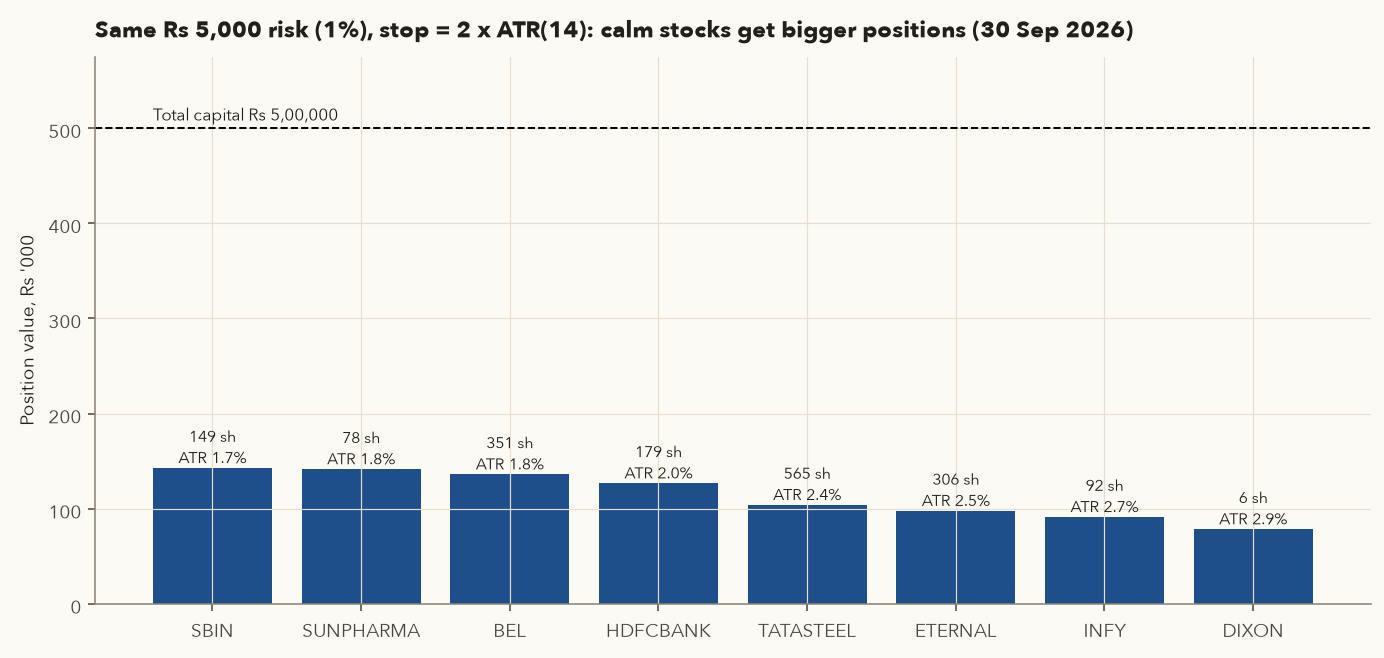
In the table below the stop is placed 2 × ATR(14) below the close. ATR(14), the Average True Range, is the average daily trading range over the last 14 sessions including overnight gaps (Wilder's method, Chapter 4); Section 9.3 uses it for sizing.
Same rupees in, very different rupees at risk
| Stock | Close | Shares for ₹1 lakh | Loss if stopped (2 ATR) |
|---|---|---|---|
| SBIN | 959.50 | 104 | ₹3,477 |
| SUNPHARMA | 1,816.60 | 55 | ₹3,522 |
| BEL | 388.30 | 257 | ₹3,657 |
| HDFCBANK | 708.70 | 141 | ₹3,935 |
| TATASTEEL | 184.30 | 542 | ₹4,791 |
| ETERNAL | 320.00 | 312 | ₹5,089 |
| DIXON | 13,100.00 | 7 | ₹5,270 |
| INFY | 994.10 | 100 | ₹5,386 |
The risk differs by 55% between SBIN and INFY for the "same" position. Over many trades, your results end up driven by whichever stocks happened to be volatile.
9.2 Percentage risk: the 1–2% rule
This is the method most professionals use and the one this course recommends. Varsity notes that professional traders rarely risk more than 1–3% of capital on one trade. You decide the maximum loss per trade as a percentage of equity, and the distance to your stop then sets the quantity.
- Equity
- Your trading capital in ₹, measured by one of the models in Section 8 (core equity for a beginner).
- risk%
- The most you are willing to lose on this one trade, as a % of equity: 1% in this course's examples.
- Risk budget
- That maximum loss in rupees.
- Entry, Stop
- Your planned buy price and stop-loss price, in ₹ per share. Entry − Stop is the rupee risk per share.
- \(\lfloor x \rfloor\)
- "Round \(x\) down to a whole number". You can't buy part of a share, and rounding up would risk more than the budget.
- max position%
- The largest share of equity you allow in one stock, for example 25%. Dividing that rupee amount by the entry price gives the most shares you may hold.
- Multiply equity by risk% to get the rupees you can afford to lose.
- Divide by the risk per share and round down. If the stop is hit, you lose about the risk budget.
- Check the position value (quantity × entry). If it is more than your maximum position, use the smaller quantity from the cap.
A winner, sized by the 1% rule
- Entry ₹1,220.00, stop ₹1,206.41 (a tight swing-low stop). Risk per share = 1,220.00 − 1,206.41 = ₹13.59.
- 1% of ₹5,00,000 = ₹5,000. Quantity = ⌊5,000 / 13.587⌋ = 367 shares. Position value = 367 × 1,220 = ₹4,47,740, which is 89.5% of the account.
- At 2% risk the formula says 735 shares = ₹8,96,700: more than the whole account. In a cash account you cannot buy that without leverage. The cap of ₹5,00,000 / 1,220 = 409 shares applies.
- Exit on 31 Aug 2026 at ₹1,272.00. Profit at 1% size = 367 × 52 = ₹19,084 = +3.83R gross (+3.61R after costs).
Lesson: a very tight stop produces a very large position. Add a maximum position size (for example 20–25% of equity per stock) as a second limit, and accept a smaller rupee risk on tight-stop trades. framework.risk.position_size(..., max_position_pct=25) does exactly this.
When the stop does not protect you: a gap
- Entry ₹273.89, stop ₹267.40. Risk per share ₹6.49. At 1% of ₹5 lakh: ⌊5,000 / 6.488⌋ = 770 shares. Planned maximum loss ≈ ₹4,996.
- 30 Jan closed at ₹268.96, just above the stop. The next session in our data (2 Feb 2026) opened at ₹251.60, 6.45% below the previous close and well below the stop.
- Actual loss = 770 × (273.89 − 251.60) = ₹17,163 = 3.43% of the account, or −3.54R after costs, three and a half times the plan.
- Across all 2,187 completed Chapter 5 trades, 89 (4.1%) exited via a gap below the stop, averaging −1.14R. Only 0.23% of trades lost more than 2R, but this one did.
This is why the 1% rule must be 1%, not 5%. At 5% risk the same gap would have cost 17% of the account in one morning.
9.3 Percentage volatility (ATR) sizing
Varsity's fourth method, from Van Tharp, sizes the position so that one average day's move (ATR) equals a fixed % of equity. It uses the Average True Range rather than standard deviation, because ATR includes gaps (Chapter 4).
- Equity
- Your trading capital in ₹.
- ATR
- The Average True Range, usually ATR(14): the average daily price range over the last 14 sessions, including overnight gaps, in ₹ per share (Chapter 4).
- \(v\%\)
- The share of equity you allow one average day's move to cost, for example 1% or 2%.
- \(m\)
- How many ATRs away from entry you place the stop (2 in this chapter's examples), so \(m \times\) ATR is the risk per share.
- risk%
- The most you will lose on the trade if the stop is hit, as a % of equity.
How it works: a volatile stock has a large ATR, so you buy fewer shares, and a calm one gets more. Either way, one normal day's move (first version) or a stop-out (second version) costs the same share of your account. Round the result down to whole shares. The second version is just the percentage-risk rule with the stop set at \(m\) ATRs.
ATR sizing step by step
- SBIN close ₹959.50, ATR(14, Wilder) = ₹16.71 (1.74% of price).
- Varsity-style with \(v=2\%\): ₹10,000 / 16.71 = 598 shares = ₹5,73,781. Too big for a ₹5 lakh cash account. With \(v=1\%\): 299 shares = ₹2,86,890.
- Combined with a 2×ATR stop and 1% risk: stop = 959.50 − 2 × 16.71 = ₹926.07. Risk per share ₹33.43. Quantity = ⌊5,000 / 33.43⌋ = 149 shares (₹1,42,966, 28.6% of the account).
9.4 Equity-curve sizing
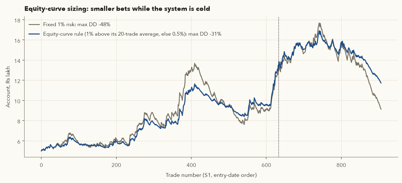
A refinement used by many systematic traders: risk your normal % while your account's equity curve is healthy, and cut size (for example in half) when the equity curve drops below its own moving average. The logic: losing streaks cluster when a system is out of sync with the market (Section 13), so betting less during those stretches limits the damage, and you return to full size once results recover.
1% fixed vs "1%, or 0.5% when below the 20-trade average equity"
- Fixed 1%: the account multiplied by 1.83 overall, with a maximum drawdown of −48.3%. From 2024, when S1's edge turned negative, it lost 29.5%.
- Equity-curve rule: multiplied by 2.35, maximum drawdown −30.6%, and only −12.1% from 2024.
The rule helped here because S1's losses came in a long cluster. It is not magic: in choppy periods it can cut size just before a recovery. Test it on your own system (Chapter 12) before relying on it.
10. Position sizing for futures lots
Futures add two complications: you trade in whole lots, and the margin is a small fraction of the exposure. Margin is what the exchange asks you to deposit. It is not your risk. Size by the rupee loss at your stop, exactly as for shares, and then check that the margin fits.
- Equity × risk%
- Your rupee risk budget for the trade, as in Section 9.2.
- Entry − Stop
- The distance to your stop, in ₹ (or index points) per unit.
- Lot size
- Units per futures contract: 65 for Nifty, 750 for SBIN, 500 for RELIANCE.
- (Entry − Stop) × Lot size
- The rupee loss on one lot if the stop is hit.
- \(\lfloor x \rfloor\)
- Round down to a whole number. Here it can come out as 0.
- Work out what one lot loses if the stop is hit.
- Divide your risk budget by that and round down. That is the number of lots. A result of 0 means even one lot is too big for your account.
- Flip it round to see how much equity one lot needs: the loss per lot divided by your risk% (as a decimal, 1% = 0.01). The last two columns of the table below are these two steps for a 2×ATR stop.
What one lot really risks
| Contract | Fut close | Lot | Notional ₹ | Margin ₹ | Leverage | ATR(14) | 2-ATR stop loss per lot ₹ | Equity needed at 1% risk ₹ |
|---|---|---|---|---|---|---|---|---|
| NIFTY | 22,707.30 | 65 | 14,75,974 | 1,67,370 | 8.82× | 209.03 | 27,173 | 27,17,300 |
| SBIN | 967.20 | 750 | 7,25,400 | 1,28,274 | 5.66× | 16.71 | 25,071 | 25,07,100 |
| TATASTEEL | 186.07 | 2,750 | 5,11,692 | 90,454 | 5.66× | 4.42 | 24,319 | 24,31,900 |
| INFY | 1,002.60 | 400 | 4,01,040 | 77,008 | 5.21× | 26.93 | 21,543 | 21,54,300 |
| RELIANCE | 1,191.80 | 500 | 5,95,900 | 1,05,706 | 5.64× | 20.25 | 20,248 | 20,24,800 |
| HDFCBANK | 715.55 | 650 | 4,65,107 | 82,137 | 5.66× | 13.96 | 18,142 | 18,14,200 |
Margin = SPAN margin (the exchange's estimate of a worst-case one-day loss, from NSE Clearing's SPAN file) + extreme-loss margin (2% of notional for index futures, 3.5% for stock futures; see Chapter 9). The ATR used is the underlying's daily ATR. Stock ATRs are from the cash market, Nifty's from the index.
With a normal swing stop (2×ATR), one lot of any of these contracts risks ₹18,000–₹27,000. At 1% risk per trade you need roughly ₹18–27 lakh of trading capital per lot. With ₹10 lakh at 2% risk, only HDFCBANK (₹18,142 per lot ≤ ₹20,000) fits, and only 1 lot. Having enough margin to open a position does not mean you can afford it. If your account is smaller, the right futures position is usually zero: trade the cash market, or wait. Index lot sizes were set large on purpose (SEBI's minimum contract value rules), and the numbers above show the effect.
Leverage turns ordinary bad days into account events
- Largest Nifty one-day fall in 2025–Sep 2026: −3.26% on 19 Mar 2026. On one lot (notional ₹14,75,974 at 30 Sep 2026 prices) that is −₹48,147, which is 28.8% of the ₹1,67,370 margin in a single day.
- On 23 Mar 2020 the Nifty fell 12.98%. At today's 8.82× leverage that is −114% of margin: more than the entire deposit in one session, before you could act.
- Risk on margin = index move × leverage. A 1% Nifty move is ₹14,760 per lot, 8.8% of margin.
10.1 Varsity's percentage-margin model
For futures, Varsity also describes capping the margin used per position at a fixed % of equity (for example 20%), and pairing it with the core or reduced-total equity model.
Which contracts fit?
- 20% of ₹5,00,000 = ₹1,00,000. NIFTY (₹1,67,370) does not fit. RELIANCE (₹1,05,706) does not fit. INFY (₹77,008) fits: take 1 lot.
- Core equity is now 5,00,000 − 77,008 = ₹4,22,992. 20% of that = ₹84,598. HDFCBANK (₹82,137) fits. TATASTEEL (₹90,454) does not.
- Now check risk: INFY + HDFCBANK at 2×ATR stops = ₹21,543 + ₹18,142 = ₹39,685 at risk, which is 7.9% of the account. The margin rule alone allowed far more risk than the 1–2% rule would. Margin caps are a ceiling, never the sizing method.
11. R-multiples, expectancy and the break-even win rate
Once every trade risks a planned amount, you can measure results in R, units of initial risk. This makes trades of different sizes and prices comparable, and turns a trading method into numbers you can test.
- Entry, Exit, Stop
- Your buy price, sell price and initial stop-loss, in ₹ per share. Entry − Stop is the planned risk per share, called 1R.
- \(R\)
- The trade's result measured in units of that risk. +2R means you made twice what you risked. −1R is a clean stop-out. Worse than −1R means the price gapped through the stop. (For a short trade, flip the signs: \((\text{Entry} - \text{Exit})/(\text{Stop} - \text{Entry})\).)
- \(W\)
- The win rate: the fraction of trades that made money (0.415 = 41.5%). \(1 - W\) is the loss rate.
- \(\overline{R}_{\text{win}}\)
- The average R of the winning trades.
- \(\overline{R}_{\text{loss}}\)
- The average size of the losing trades in R, written as a positive number (0.95 for an average loss of −0.95R).
- \(E\)
- The expectancy: the average R per trade over many trades. It equals the simple average of all the R-multiples.
- RR
- The payoff ratio (reward : risk): \(\overline{R}_{\text{win}} / \overline{R}_{\text{loss}}\).
- Break-even win rate
- The win rate at which \(E = 0\): win less often than this and the system loses money.
- Profit factor
- Total of all winning trades divided by the total of all losing trades (ignoring the minus sign, which is what \(|\ldots|\) means). Above 1 means the system made money.
- Convert each trade to R: its profit per share divided by its planned risk per share.
- Split the trades into winners and losers. Work out the win rate and the average R of each group.
- Expectancy = win rate × average win − loss rate × average loss. Multiply by your rupee risk per trade (1R) to see the average ₹ per trade.
- Set \(E = 0\) and solve for \(W\) to get the break-even win rate. Compare it with your actual win rate: the gap is your margin of safety.
Computing R
\(R = (1272.00 - 1220.00)/(1220.00-1206.41) = 52.00/13.59 = 3.83\). After brokerage, STT and other costs (Chapter 13) the net result was 3.61R. In rupees at 1% risk: about 3.61 × ₹5,000 ≈ ₹18,000.
Expectancy of four real swing setups
| Setup | Trades | Win rate | Avg win | Avg loss | Payoff (RR) | Expectancy | Break-even win% | Profit factor | 2024–26 expectancy |
|---|---|---|---|---|---|---|---|---|---|
| S1 Trend pullback | 906 | 38.3% | 1.76R | 0.96R | 1.83 | +0.080R | 35.4% | 1.13 | −0.120R (273) |
| S2 52-wk breakout | 418 | 37.8% | 1.42R | 0.84R | 1.68 | +0.012R | 37.3% | 1.02 | −0.268R (108) |
| S3 Support bounce | 169 | 40.2% | 2.01R | 1.11R | 1.81 | +0.147R | 35.5% | 1.22 | +0.019R (61) |
| S4 Weekly + daily | 694 | 41.5% | 2.06R | 0.95R | 2.16 | +0.295R | 31.7% | 1.53 | −0.100R (201) |
- S4 by hand: \(E = 0.415\times2.0557 - 0.585\times0.9532 = 0.8531 - 0.5576 = +0.2954R\) per trade.
- Break-even win rate for S4 = 0.9532 / (2.0557 + 0.9532) = 31.7%. It actually won 41.5%: a cushion of almost 10 points.
- S2 won 37.8% against a break-even of 37.3%. Its edge was razor-thin even before 2024, and negative since.
- In rupees, at 1% risk on ₹5 lakh, 1R = ₹5,000. S4's +0.295R is about ₹1,477 per trade on average. No single trade pays that: each one is either a loss of about ₹4,766 (0.9532R) or a win averaging about ₹10,279 (2.0557R). Expectancy only shows up as an average over many trades.
Note that every setup wins less than half the time and still made money over the full period. Win rate alone tells you almost nothing. Win rate together with payoff tells you everything.
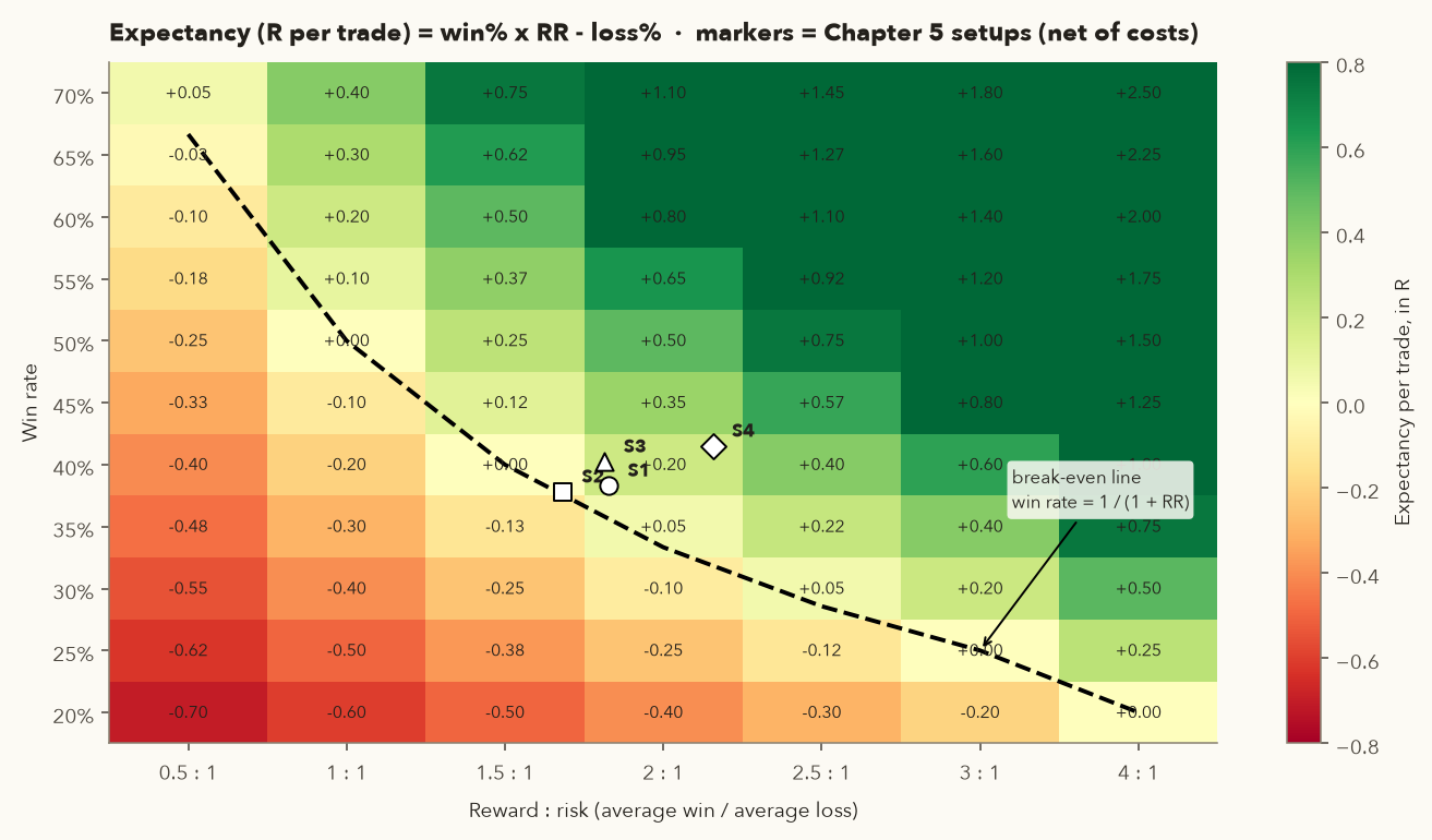
Win rate vs reward:risk: break-even and expectancy
| Reward : risk | Break-even win rate | Expectancy at 30% wins | at 40% | at 50% | at 60% |
|---|---|---|---|---|---|
| 0.5 : 1 | 66.7% | −0.55R | −0.40R | −0.25R | −0.10R |
| 1 : 1 | 50.0% | −0.40R | −0.20R | 0.00R | +0.20R |
| 1.5 : 1 | 40.0% | −0.25R | 0.00R | +0.25R | +0.50R |
| 2 : 1 | 33.3% | −0.10R | +0.20R | +0.50R | +0.80R |
| 3 : 1 | 25.0% | +0.20R | +0.60R | +1.00R | +1.40R |
Read across a row: at 2:1, a 30% win rate loses 0.10R per trade, while 40% earns +0.20R. Read down a column: at a 40% win rate you need better than 1.5:1 just to break even. Every expectancy here is before costs and slippage, which cost the Chapter 5 setups 0.05–0.10R per trade, so a setup needs a clear margin above its break-even line.
- Too few trades. 20 trades tell you almost nothing. You want 100+ before trusting a number, and even then the 2024–26 column shows edges can fade.
- Ignoring costs. In the Chapter 5 trades (median stop distance 4.1% of price), delivery costs averaged 0.07R per trade for S1. Before costs S1 earned about +0.15R per trade, so costs ate almost half of its edge. Tight stops make costs larger in R terms.
- Chasing win rate. Moving targets closer raises the win rate and usually lowers expectancy (Section 15 shows this with real trades).
12. Kelly criterion and half-Kelly
The Kelly criterion, which Varsity covers in chapter 14, answers: given my edge, what fraction of capital should I bet to grow fastest over the long run? Bet too little and you grow slowly. Bet too much and the losses (which hurt more than equal-sized gains help, Section 7) drag growth down and eventually into ruin.
- \(K\)
- The Kelly fraction: the share of capital to risk per trade (the loss if the stop is hit) that grows the account fastest in the long run. 0.144 means risk 14.4% per trade. Negative means don't trade.
- \(W\)
- The win rate, as a fraction.
- RR
- The payoff ratio: average win ÷ average loss, both in R or both in ₹.
- \(f\)
- Any fraction of capital you might risk per trade (0.01 = 1%).
- \(R\)
- One trade's result in R-multiples (Section 11). \(1 + f \cdot R\) is what the account is multiplied by after that trade: risking 1% on a +2R trade gives × 1.02.
- \(\ln\)
- The natural logarithm. Taking logs turns a chain of multiplications into a sum, so averaging them measures compound growth.
- \(\mathbb{E}[\ldots]\)
- "Expected value": the average over all your trades.
- \(\arg\max_f\)
- "The value of \(f\) that makes \(g(f)\) largest."
- Formula version: plug the win rate and payoff ratio into the first line. It assumes every win and every loss is exactly the average size.
- Real-trades version: for each candidate \(f\), compute \(\ln(1 + f \cdot R)\) for every past trade and average them. That is the growth rate per trade at that bet size.
- The \(f\) with the highest growth is the Kelly bet. Risk more than that and growth falls; well beyond it, the account shrinks.
framework.risk.kelly_fraction(win_rate, win_loss_ratio)returns the formula value. Treat it as a ceiling, not a target.
Formula vs reality
- \(W = 0.415\), RR = 2.0557 / 0.9532 = 2.1566.
- \(K = 0.415 - 0.585/2.1566 = 0.415 - 0.2713 = 0.1437\). The formula says risk 14.4% of capital per trade.
- The formula assumes every win is exactly +2.06R and every loss exactly −0.95R. Real outcomes vary (some wins +8R, some gap losses −3R). Maximising the actual average log-growth over the 694 real trades gives an optimum of 9.4%, and growth turns negative beyond about 20.3%.
- For S1: formula 4.5%, empirical optimum 3.2%. For S4 trades from 2024 on, the formula gives −6.7%. Negative Kelly means the right bet size is zero.
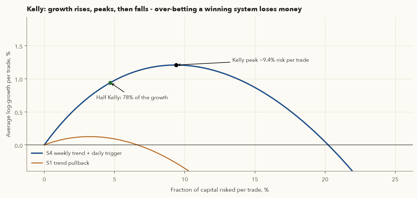
Why even half-Kelly is too much for a person
| Sizing | Risk per trade | Median ending multiple | Median max drawdown | P(drawdown ≥ 50%) |
|---|---|---|---|---|
| Full Kelly | 9.4% | 9.82× | −80.1% | 99.7% |
| Half Kelly | 4.7% | 6.10× | −51.6% | 55.5% |
| Quarter Kelly | 2.35% | 3.02× | −29.4% | 3.9% |
| Fixed 1% | 1.0% | 1.69× | −13.5% | 0.0% |
Full Kelly maximises long-run growth, and along the way it puts you through a near-certain 50%+ drawdown. And this assumes the edge is known and stable. S4's edge was not: from 2024 it was negative. Kelly computed on a past edge that later shrinks means you were overbetting.
Use Kelly as an upper bound and a sanity check, not a sizing rule. If your Kelly estimate is below your planned risk %, you are overbetting: cut size. If Kelly is near zero or negative on recent trades, stop trading that setup. Varsity suggests combining Kelly with the percentage-risk method. A practical version: risk = min(1–2%, ¼ Kelly). framework.risk.kelly_fraction(win_rate, win_loss_ratio) returns the formula value.
13. Drawdowns, losing streaks and risk of ruin
13.1 Same trades, different bet size
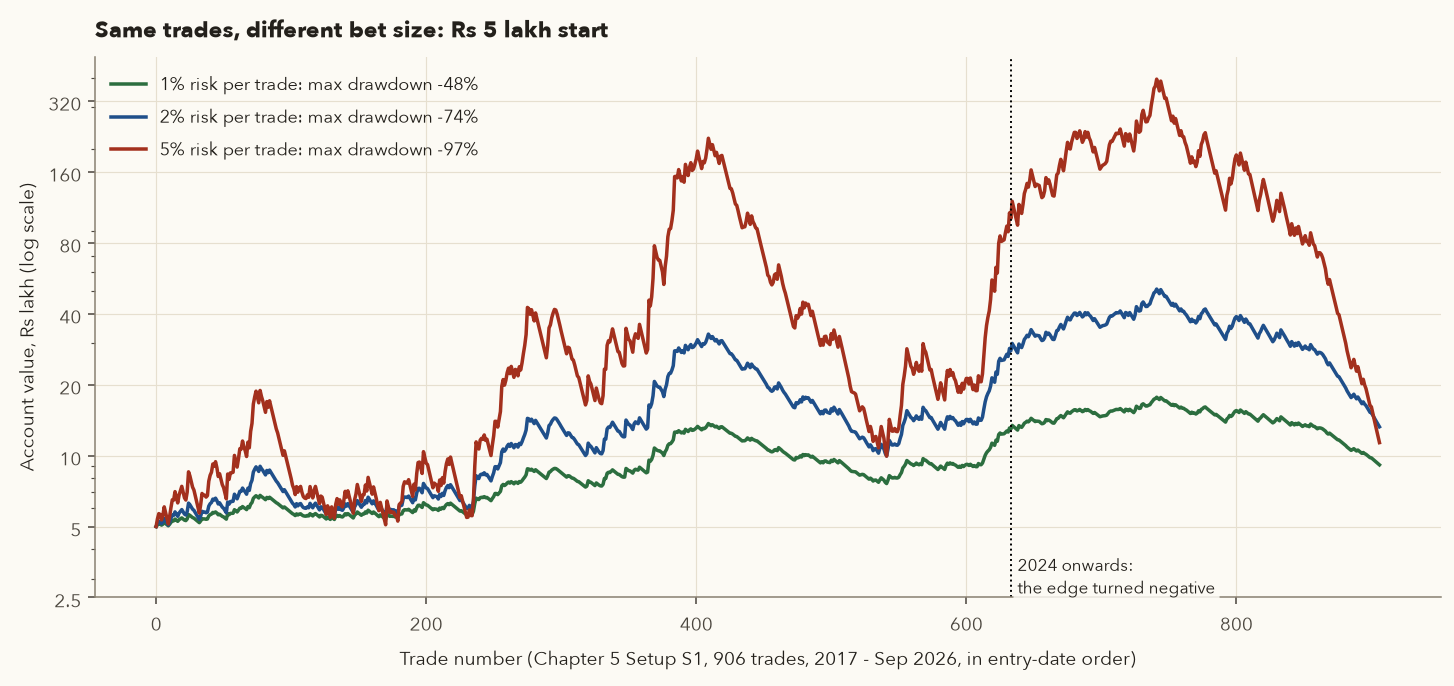
Here is the most important experiment in this chapter. Take the exact same 906 S1 trades in the order they happened (2017 – Sep 2026) and replay them risking 1%, 2% and 5% of current equity per trade.
How the drawdown happened
S1's first trade of 2024 was trade no. 634. From 2024 the setup's net expectancy was −0.120R over 273 trades, and it included a run of 16 consecutive losses (entries 23 Feb to 27 May 2026). At 1% risk, 16 straight losses of about 1R cost roughly \(1-0.99^{16}\approx 15\%\). At 5% they cost \(1-0.95^{16}\approx 56\%\). In August–September 2026, 27 of 28 trades across all four setups lost, a combined −23.29R. This is what "the edge turned negative" looks like from inside: no single disaster, just a steady drip of losses.
13.2 Monte Carlo: what could have happened
One historical sequence is one possible path. A Monte Carlo simulation reshuffles your real trade results thousands of times to show the range of paths your system could produce. We drew 200 trades at random (with replacement) from S1's 906 net-R outcomes, 10,000 times, at each risk level.
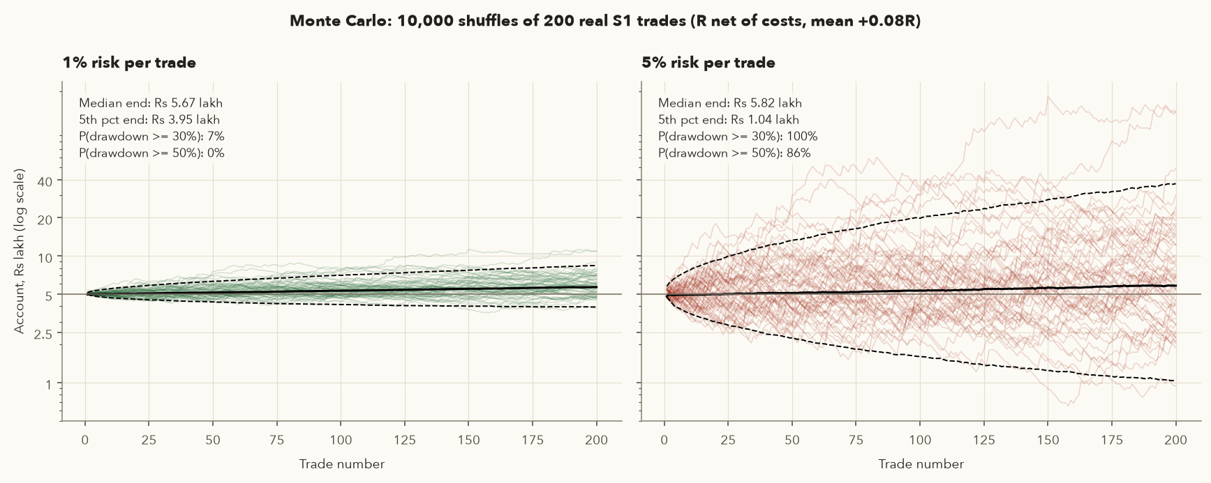
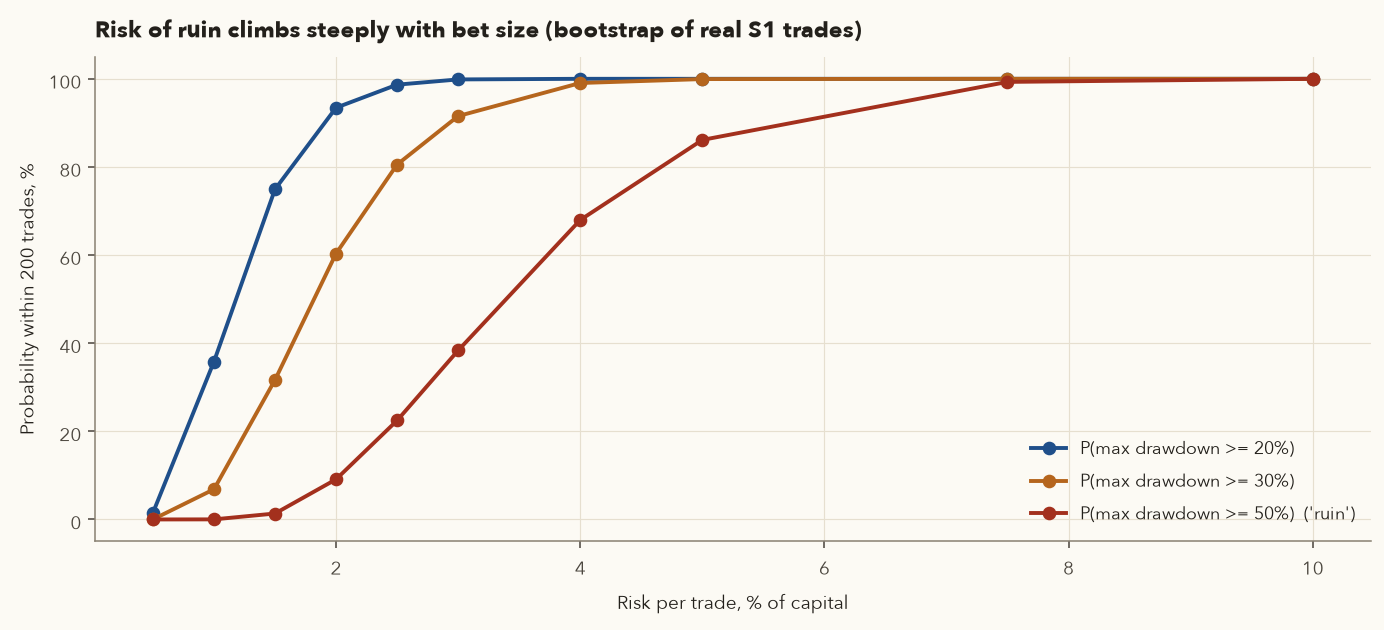
| Risk per trade | Median end (× start) | 5th pct end | Median max DD | P(DD ≥ 20%) | P(DD ≥ 30%) | P(DD ≥ 50%) | P(lose money) |
|---|---|---|---|---|---|---|---|
| 0.5% | 1.07 | 0.89 | −9.0% | 1.5% | 0.0% | 0.0% | 26.9% |
| 1% | 1.13 | 0.79 | −17.5% | 35.8% | 6.9% | 0.0% | 28.8% |
| 1.5% | 1.18 | 0.69 | −25.3% | 74.9% | 31.7% | 1.4% | 30.7% |
| 2% | 1.22 | 0.60 | −32.6% | 93.4% | 60.3% | 9.1% | 32.5% |
| 3% | 1.26 | 0.44 | −45.6% | 99.9% | 91.5% | 38.4% | 36.2% |
| 5% | 1.16 | 0.21 | −66.0% | 100% | 99.9% | 86.1% | 44.3% |
| 10% | 0.47 | 0.02 | −92.2% | 100% | 100% | 100% | 64.0% |
Three things to read from this table:
- Beyond about 3% risk, more risk does not even raise the typical outcome. The median ending at 10% (0.47×) is below the median at 0.5%. Over-betting a positive edge destroys it, which is the Kelly curve again.
- Drawdowns are larger than intuition suggests. Even at 1%, there is a 36% chance of a 20% drawdown within 200 trades. Decide now that a 20% drawdown at 1% risk is "normal bad", not a reason to abandon a tested plan.
- A positive edge still loses money 27–29% of the time over 200 trades at low risk. A thin edge needs many trades to show itself. Re-run with S1's 2024–26 trades only (mean −0.12R): at 1% risk the median ending is 0.77× and 92% of paths lose money. A negative edge cannot be fixed by sizing.
What "risk of ruin" means here. Risk of ruin is the probability that a run of losses takes your account down to a level from which you cannot or will not carry on. If you always risk a fixed percentage of current equity, the account never mathematically reaches zero (each loss is a slice of a smaller pie), so the textbook "probability of losing everything" is not the useful number. In practice, traders quit, change systems or start revenge trading long before zero. So we define ruin as a 50% drawdown (which then needs +100% to repair) and measure its probability by simulation, as in the table above.
13.3 Losing streaks are normal
- \(P(\ldots)\)
- "The probability that …", as a fraction between 0 and 1.
- \(W\)
- The win rate, so \(1 - W\) is the chance that any one trade loses (0.62 for a 38% win rate).
- \(k\)
- The length of the losing streak, in trades.
- \((1-W)^k\)
- The loss chance multiplied by itself \(k\) times. This assumes each trade is independent of the last.
How it works: this is the chance that a particular run of \(k\) trades, such as the next 8, all lose. The chance of seeing at least one such streak somewhere in \(n\) trades is much higher, because there are many places in the sequence where it could start. That figure has no simple formula. It is computed by simulation or dynamic programming (as in our script).
How often do long streaks occur?
- Win rate 38% (S1-like): probability that a given 8 trades all lose = \(0.62^8 = 2.2\%\). But the probability of at least one streak of 8+ somewhere in 100 trades is 57%. 10+ in a row: 26%.
- Win rate 50%: 8+ in a row within 100 trades: 17%. Win rate 60%: 5+ in a row: 46%.
- S1's real worst streak was 16. At its 38.3% win rate, a 16-streak somewhere in 906 trades has about a 14% chance. Unlucky, but not impossible, and it coincided with the edge fading.
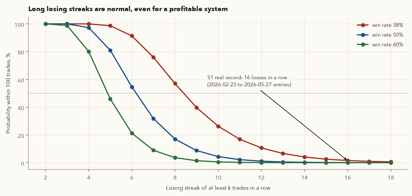
Before you trade a system, write down: "With my win rate, a streak of k losses is likely. At my risk %, that costs X%." For S1 at 1%: 8 losses ≈ 7.7%, 10 losses ≈ 9.6%. If that number would make you quit or double up, reduce risk until it would not.
14. Portfolio heat, correlation risk and sector limits
The 1% rule controls one trade. Portfolio heat controls all of them together:
- \(i\)
- Labels each open position: position 1, 2, 3 and so on.
- \(\text{qty}_i\)
- The number of shares (or units) held in position \(i\).
- \(\text{entry}_i - \text{stop}_i\)
- How much each share loses, against what you paid, if the stop is hit, in ₹. For a short position, use stop − entry.
- \(\max(0,\ \dots)\)
- "The larger of 0 and the bracket". Once a stop sits at or above the entry price (below it, for a short), hitting it loses none of your capital, so that position counts as 0.
- Equity
- Your account capital in ₹.
- \(\sum_{\text{open positions}}\)
- Add the result up across every open position.
- Heat
- The share of your capital you would lose if every stop were hit at once, as a %.
How it works: for each open trade, multiply the quantity by the distance from entry down to its current stop to get the rupees of capital at risk. Add them up and divide by equity. Five positions each sized at 1% risk give a heat of about 5%. Move a stop to breakeven and that position drops out of the total.
Heat is the total you would lose if every stop were hit at once. Typical caps: 4–6% for swing traders (for example 5 positions × 1%), lower in a weak market regime. Once a stop is moved to breakeven or above, that position's heat drops to zero, and that is how you make room for new trades.
Heat counts only losses to your own capital. It ignores open profit you could give back: a stock up 15% with its stop at breakeven has zero heat but can still hand back that 15%. Track that separately as open profit at risk, qty × (current price − stop), and trail stops on big winners so it stays reasonable.
Five "different" trades, one bet
- On 21 Sep 2026, S4 triggered five long entries at once: BAJFINANCE, TRENT, PIDILITIND, CDSL and HAL. Five different sectors on paper.
- Heat at 1% each = 5%. The Nifty then fell from 23,346.40 (18 Sep) to 22,620.45 (30 Sep), −3.11%, and India VIX rose 22.6% on 24 Sep.
- All five hit their stops between 24 and 29 Sep: −1.071R, −1.064R, −1.045R, −1.029R, −1.044R. Total −5.25R = −₹26,270 on a ₹5 lakh account at 1% risk.
- The heat cap worked as designed: the loss was painful but bounded. At 3% per trade the same week would have cost about 15.8%.
All long positions share market risk. When the market turns, correlations jump and the stops get hit together, whatever the sector labels say.
14.1 Practical limits that work
| Limit | Swing trader (₹5–25 lakh) | Long-term investor | Futures trader |
|---|---|---|---|
| Risk per trade / position | 0.5–1% (max 2%) | Thesis-based; position cap does the work | 0.5–1% of total capital per lot-position |
| Max position size | 20–25% of equity | 8–10% at cost, trim above 15% | Margin ≤ 20% of equity per position |
| Portfolio heat | ≤ 5–6% (≤ 3% in risk-off regime) | n/a (use drawdown plan) | ≤ 4% including overnight gap allowance |
| Sector / correlated cluster | ≤ 2 open trades or 2% heat per sector | ≤ 25–30% per sector | Count index + bank-stock futures as one cluster |
| Total margin used | n/a | n/a | ≤ 40–50% of capital, the rest kept as a buffer for daily mark-to-market (M2M) losses |
| Circuit breaker | Stop trading after −6% in a month; halve size after −10% from peak | Review (not panic) after a 20% portfolio fall | Pause after 3 losing trades in a row or −5% of capital in a week (count open M2M losses, not just closed trades) |
These are educational starting points, not universal truths. Write your own numbers into your plan (Section 17) and test them with the Monte Carlo above.
- Losses compound against you: −20% needs +25% to recover, −50% needs +100%. Keep drawdowns shallow.
- Quantity = (equity × risk%) ÷ (entry − stop), then cap the position size. Risk 0.5–1% per trade while learning.
- Futures: size by the rupee loss at your stop, not by margin. With a normal swing stop one lot risks ₹18,000–27,000, so you need roughly ₹18–27 lakh per lot at 1% risk. Otherwise the right number of lots is zero.
- Expectancy = win rate × average win − loss rate × average loss. A 40% win rate is fine if the winners are about twice the losers.
- Kelly is a ceiling, not a target. The same trades at 5% risk went up 79× and then lost 97%. At 1% they survived.
- Losing streaks of 8+ are normal at a 38% win rate, and correlated trades get stopped out together. Cap total portfolio heat.
15. Trading psychology: the biases that cost money
Everything above assumes you will follow your rules. Most traders do not, at least not when it matters. Varsity's last two chapters and its Innerworth module describe the mental shortcuts (cognitive biases) that push otherwise sensible people into bad decisions. Biases are not character flaws. They are built into how human brains handle uncertainty, so trying harder doesn't remove them. Written rules that act before the bias does are what works.
15.1 Loss aversion and the disposition effect
Loss aversion: a loss hurts roughly twice as much as an equal gain pleases. In trading it shows up as the disposition effect: we sell winners too early (to "lock in" the good feeling) and hold losers too long (to avoid making the loss "real"). That is the exact opposite of what a trend-following edge needs.
What "booking profits early, giving losers room" does to a real edge
| Behaviour | Expectancy per trade |
|---|---|
| Follow the rules (as backtested, net of costs) | +0.080R |
| Take profit at +1R on every winner ("book it before it goes away") | −0.270R |
| Let full stop-outs run 50% further ("give it room") | −0.196R |
| Both habits together | −0.546R |
Why so dramatic? Only 24.5% of trades ended above +1R, but the part of those wins beyond the first 1R added up to +317.1R, more than four times the setup's total net profit of +72.3R. Meanwhile 50.3% of trades were full stop-outs. The edge lives in a few big winners and many small, controlled losers. Cutting the winners short and letting the losers run turns a positive system into a strongly negative one.
How the replay was done: our trade list has only each trade's final R, not its path, so "take profit at +1R" here caps every trade that finished above +1R at exactly +1R, and "give it room" multiplies every full stop-out (R below −0.9) by 1.5. A real +1R target would also have rescued some trades that touched +1R and then fell back, so the true damage would be somewhat smaller than −0.270R, but the direction and the scale of the problem are the same.
Rules that counter it: place the stop as a real order at entry. Never widen a stop (only tighten). Exit by rule (trailing stop, close below 20 EMA, time stop), not by feel. Review "early exits" as rule breaks in your journal.
15.2 Overconfidence and attribution bias
After a run of wins we overrate our skill and raise size. That is exactly when a regime change does the most damage. Varsity's attribution bias is the mirror image: wins are "my skill", losses are "bad luck / operators / the market was irrational". Both stop you learning.
The 5% trader in September 2024
On the real S1 sequence, a 5%-per-trade trader had turned ₹5 lakh into about ₹3.95 crore (79×) by trade no. 741 (closed 19 Sep 2024), about 20× of it before 2024 and the rest in 2024's strong run. Anyone would have felt like a genius. The next 165 trades took the account down 97%. Nothing about the method changed. The market did, and the size was far too large to survive it.
Rules: increase risk % only by written rule (for example, after 100 live trades with positive expectancy, from 0.5% to 1%), never after a hot streak. Track your live expectancy against your backtest. In the journal, label every loss as "followed plan" or "broke plan". A loss on a followed plan is a cost of business, not bad luck.
15.3 Confirmation bias
Once we own a stock we look for news that supports it and skip the rest. Varsity's example is the trader who reads only bullish reports on a stock he holds. The effect: stops get "reconsidered", warning signs get explained away, and position sizes creep up.
Rules: before entry, write one sentence on what would prove me wrong. That sentence becomes the stop. For investments, write the bear case alongside the bull case (Chapter 8) and list 2–3 measurable "thesis-broken" triggers (e.g. two consecutive quarters of falling ROCE, promoter pledge rising). Run a pre-mortem: "It's 6 months later and this lost 30%. What happened?"
15.4 Recency bias
We weight the last few weeks far more than the last few years. After a strong run every dip "will be bought". After a crash every rally "is a trap". Varsity's antidote is to keep the bigger picture in view.
Optimisers and traders both fall for it
- The efficient-frontier optimiser in Section 5, fed Oct 2022 – Sep 2024 data, piled 42% into SUNPHARMA because it had just returned 38.9% a year. It then returned −8.9% a year. That is recency bias in algorithmic form.
- S4 averaged +0.30R per trade over 2017–2026. A trader who joined in 2024 saw −0.10R and might call it "broken". A trader who joined in 2020 might have tripled their risk. Both draw conclusions from too short a window. The answer is a pre-defined review rule (Section 16), not a feeling.
15.5 Anchoring
We fix on a reference number, usually a past high or our purchase price, and judge everything relative to it. "It was ₹4,500, now it's ₹3,600, it must be cheap." The market does not know or care what you paid or where the stock used to trade.
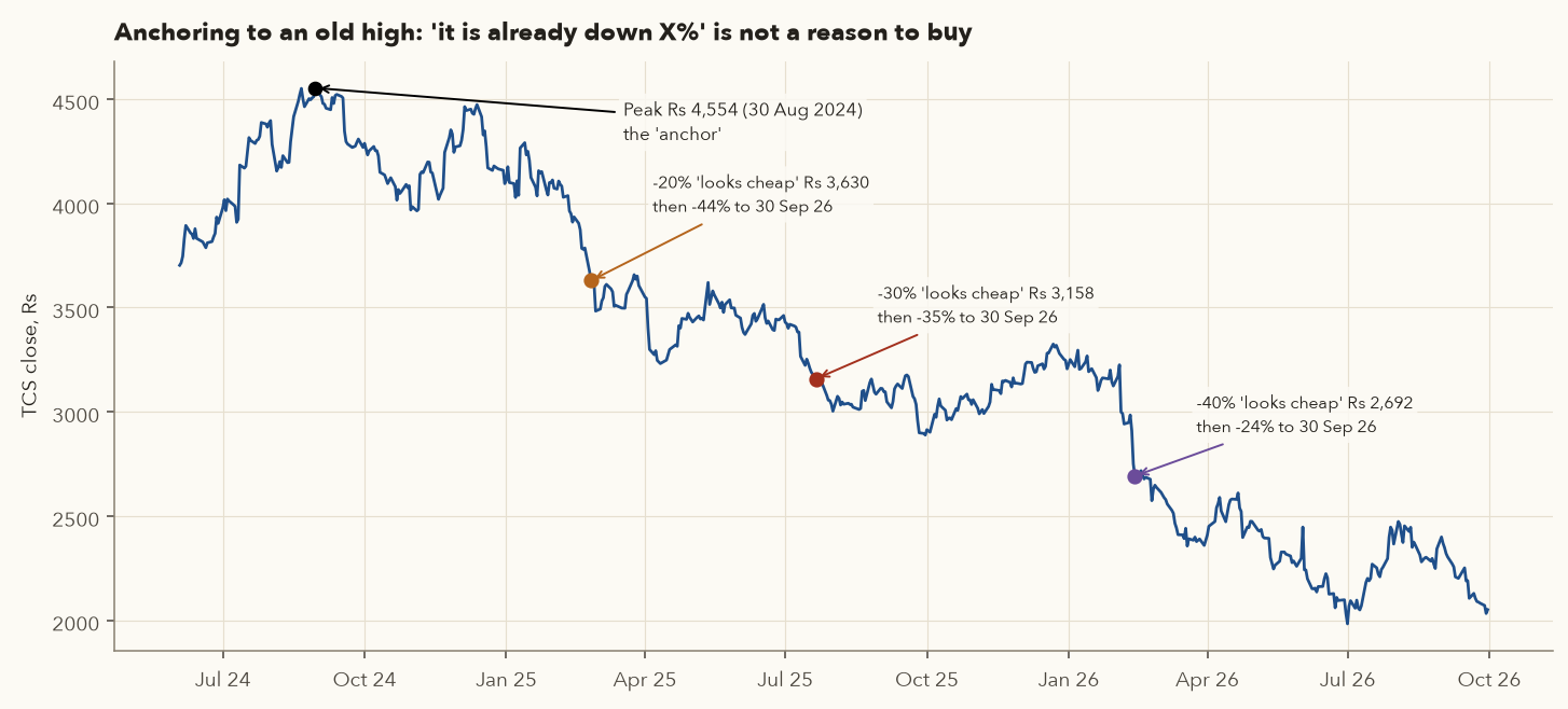
Rules: judge a stock on its own current trend (Chapters 3–5) and valuation (Chapter 8), never on its distance from a past high. Never average down a losing trade. If an investment is to be added to on a fall, that must be pre-planned in the thesis, with a fresh valuation, not a reaction to the price.
15.6 FOMO and the bandwagon (herd) effect
Fear of missing out: a stock everyone is talking about has run, and you buy because you cannot bear to watch it go higher without you. Late buyers tend to arrive after the move, with stops far away or no stops at all.
Popular, then painful
| Stock | Price 1 year before peak | Peak (date) | 1-year run-up | Then fell (to trough) |
|---|---|---|---|---|
| DIXON | ₹6,271.5 | ₹18,940.2 (17 Dec 2024) | +202% | −48.9% |
| IRCTC | ₹624.3 | ₹1,126.0 (22 May 2024) | +80% | −59.8% |
| ADANIENT | ₹2,445.1 | ₹3,645.2 (3 Jun 2024) | +49% | −51.8% |
Strong momentum is not a reason to avoid a stock. Trend-following setups (Chapter 5) deliberately buy strength. The difference is the process: a defined entry, a stop that limits the loss to 1R, and a size from Section 9. FOMO buying skips all three.
Rules: no trade without a setup from your plan. If you "missed it", write it on a watchlist and wait for a pullback setup. Mute social media and tips during market hours.
15.7 Revenge trading and the gambler's fallacy
After a painful loss, the urge is to "win it back" immediately, with a larger size, a lower-quality setup, or an instrument you don't normally trade (often options near expiry). Varsity's poker story is a revenge-trading story. It pairs naturally with the gambler's fallacy (Section 7): "I've lost four in a row, the next one must work."
Rules: a daily loss limit (e.g. 2% or 2R): hit it and you are done for the day. A cooling-off rule: after any loss above 2R, or three losses in a row, no new trades until the next session and a journal entry. Size never increases after a loss.
15.8 Illusion of control, functional fixedness and hindsight
- Illusion of control (Varsity ch. 15): piling indicators, timeframes and data feeds onto a chart because it feels like more control. More data is not more information. Chapter 4 showed most indicators are transforms of the same price series. Rule: at most 2–3 tools per setup, each with a defined job.
- Functional fixedness (Varsity ch. 16): using a tool only the way you first learned it (RSI above 70 = sell, always), and being blind to other uses or to when it stops working. Rule: know the logic behind each tool, as this course has tried to teach, so you can tell when the context has changed.
- Hindsight bias: after the fact, the move "was obvious". It makes you overconfident about predicting the next one and harsh about past decisions that were sound but unlucky. Rule: judge decisions by whether they followed the plan, not by the outcome of a single trade.
| Bias | Symptom you'll notice | Written rule that counters it |
|---|---|---|
| Loss aversion / disposition | Moving stops lower; "it will come back"; booking +0.5R winners | Hard stop order at entry; stops only tighten; rule-based exits |
| Overconfidence / attribution | Raising size after a streak; blaming "operators" | Size changes only by written schedule; journal "followed plan?" |
| Confirmation | Reading only bullish views on your holdings | Write the invalidation point and bear case before entry |
| Recency | Abandoning or over-betting a method after a few weeks | Evaluate only after 30+ trades / quarterly review |
| Anchoring | "It was ₹X, it's cheap now" | No averaging down trades; decisions on current trend and valuation |
| FOMO / herd | Buying a stock because it's everywhere | No setup, no trade; watchlist and wait |
| Revenge / gambler's fallacy | Bigger, faster trades after a loss | Daily loss limit; cooling-off after 2R loss or 3 losses |
| Illusion of control | Ten indicators, five timeframes | Max 2–3 tools per setup, each with a job |
16. The trading journal and review process
Your backtest says what should happen. Your journal records what did happen: what you did, why, and how it felt. Without one you cannot measure your expectancy, you cannot tell bad luck from bad execution, and every bias above goes unchecked.
16.1 What to record for every trade
| Before entry | At exit | Reflection |
|---|---|---|
| Date, symbol, setup name, timeframe Entry, stop, target, quantity Risk in ₹ and as % of equity Portfolio heat after this trade Market regime (Nifty vs 200-DMA, VIX) One-line reason + invalidation point Screenshot of the chart | Exit date and price, exit reason Costs (brokerage, STT, etc.) Net P&L in ₹ and in R MAE / MFE (worst and best price during the trade) if available | Did I follow the plan? (yes/no) If no: which rule, and why? Emotion at entry and exit (1–5 scale) What would I do differently? |
framework.journal keeps this as a CSV you own, and refuses a trade without a stop. From the project folder:
python -m framework.journal add AXISBANK --entry 1220 --stop 1206.4 --qty 367 --setup trend_pullback
python -m framework.journal close 1 --exit 1272 --reason target
python -m framework.journal stats (win rate, average win/loss in R, expectancy, profit factor, by setup).
close_trade(..., followed_plan=False, notes="moved stop") records rule breaks so you can measure what they cost you.
16.2 The review cycle
- Daily (5 minutes, after the close): update open trades and stops, compute heat, log any rule breaks. No new analysis while emotional.
- Weekly (30 minutes): review every closed trade's screenshot. Were entries per plan? Any patterns in mistakes (time of day, after losses, a sector)?
- Monthly / every 20–30 trades: compute live win rate, average R, expectancy and max drawdown. Compare with the backtest. Compute expectancy separately for "followed plan" and "broke plan" trades. That gap is the price of your indiscipline in rupees.
- Quarterly: decide changes. Only change a rule if the data (30+ trades) supports it, and change one thing at a time.
Decide this in advance, in numbers, for example: "If live expectancy over the last 50 trades is below −0.1R, or drawdown exceeds 1.5× the worst Monte-Carlo 95th-percentile drawdown, I stop, paper-trade, and re-test." For S1 at 1% risk, the 95th-percentile drawdown over 200 trades was −31.5%. After S1's equity peak (trade no. 741, Sep 2024), its 50-trade expectancy first fell below −0.1R at trade no. 780 (entry 20 Dec 2024), when the drawdown was −12.1%. Following the rule there would have avoided most of the eventual −48.3% drawdown.
17. Your written trading plan (template)
A trading plan is a one- or two-page document you write when calm and follow when not. If something isn't in the plan, you don't do it. Copy this template and fill it in. Chapter 17 turns it into your complete framework.
MY TRADING PLAN — version 1.0 — date: ________
1. Goals & capital
   Trading capital: Rs ______ (money I can lose without changing my life)
   Investment capital (separate): Rs ______   Emergency fund kept outside both: yes/no
   Realistic goal: positive expectancy over 100 trades, max drawdown under ___%

2. Markets & instruments
   Swing: NSE cash, Nifty 200 stocks, avg daily value > Rs 50 cr
   Futures: only when capital >= Rs ___ lakh per lot at 1% risk (see Section 10)
   Not traded: intraday, options buying near expiry, illiquid small caps

3. Setups (from Ch 5 / Ch 12, each backtested, with its expectancy)
   S_: __________  entry rule / stop rule / exit rule / expectancy ___R over ___ trades

4. Risk rules
   Risk per trade: ___% of core equity (start 0.5%; max 1%)
   Max position: ___% of equity      Max portfolio heat: ___%
   Max per sector / correlated cluster: ___ trades or ___% heat
   Regime: Nifty < 200-DMA -> risk halved, trend setups paused
   Futures: margin used <= ___% of capital; never add to a losing position

5. Circuit breakers
   Daily loss limit: ___R  -> stop for the day
   After 3 consecutive losses or a loss > 2R: no trade until next session + journal entry
   Monthly loss of ___% -> half size;  drawdown of ___% from peak -> stop, review, paper-trade

6. Routine
   Pre-market: check regime, events/results calendar, open positions' stops
   Entries: only at planned levels with orders placed; no chasing
   Post-close: journal, update stops, compute heat
   Weekly / monthly / quarterly reviews (Section 16)

7. Personal rules
   No trading when ill, sleep-deprived, or after a major personal upset
   No tips, no social-media trades, no changing rules during market hours

Signed: ____________   Review date: ____________
18. Stress and discipline routines
Varsity's Innerworth module comes back again and again to one theme: trading performance depends on your state of mind as much as on your method. Stress narrows attention and pushes you towards impulsive, short-term decisions, which are exactly the biases above. A few habits help:
- Treat a loss as feedback, not failure. A stopped-out trade that followed the plan is a business expense. Ask "what is this telling me?" (setup, market regime, execution) rather than "why me?".
- Be flexible and disciplined. Discipline means following the plan. Flexibility means changing the plan through the review process when data says so, never mid-trade.
- Size for sleep. If you are checking prices at night, the position is too big. Cut it until you can switch off. That is the human version of the Monte Carlo table.
- Decide before the market opens. Orders (entries, stops) placed in advance remove most in-the-moment decisions. Swing and positional trading's great advantage over intraday is that you can do your thinking when the market is closed.
- Limit screen time. Checking prices every few minutes on a swing position feeds anxiety and itchy exits. Twice a day is plenty for a daily-chart strategy.
- Physical basics matter. Sleep, exercise and an organised workspace measurably improve decision quality. Don't trade on days when you are unwell, exhausted or emotionally upset.
- Face fear and regret directly. Name the fear ("I'm afraid this gap-down will continue") and check it against the plan, instead of acting to make the feeling go away.
- Take planned breaks after a circuit breaker triggers or a big win. Both distort judgement.
19. Try it yourself
These snippets need a copy of the course repository and Python with pandas and numpy (setup steps are in its framework/README.md). Run them from the repository's root folder, for example with .venv/bin/python, because the file paths are relative to that folder. They use the course data directly. Your numbers can differ from the chapter in the second decimal: the chapter's script also drops a few zero-range holiday placeholder bars and uses population (n) rather than sample (n−1) standard deviation for the matrix example.
19.1 Correlation matrix and portfolio volatility
import pandas as pd, numpy as np
D = "data/ohlc/"
stocks = ["HDFCBANK", "INFY", "ITC", "SUNPHARMA", "TITAN"]
w = np.array([0.25, 0.20, 0.15, 0.15, 0.25])
px = pd.DataFrame({s: pd.read_csv(D + s + ".csv", index_col=0, parse_dates=True)["Adj Close"] for s in stocks})
ret = px.pct_change(fill_method=None).loc["2024-10-01":"2026-09-30"].dropna()

print(ret.corr().round(2))                       # correlation matrix
cov = ret.cov()                                  # variance-covariance matrix (daily)
port_sd = np.sqrt(w @ cov.values @ w)            # sigma_p = sqrt(w' S w)
print(f"Portfolio vol: {port_sd:.4%} per day, {port_sd*np.sqrt(252):.2%} per year")
print(f"Weighted avg of vols: {(w * ret.std()).sum()*np.sqrt(252):.2%} per year")
# -> about 0.85% per day, 13.5% per year vs ~22% weighted average
19.2 Value at Risk three ways
import pandas as pd, numpy as np
D = "data/ohlc/"
stocks = ["HDFCBANK", "INFY", "ITC", "SUNPHARMA", "TITAN"]
w = np.array([0.25, 0.20, 0.15, 0.15, 0.25])
px = pd.DataFrame({s: pd.read_csv(D + s + ".csv", index_col=0, parse_dates=True)["Adj Close"] for s in stocks})
pr = (px.pct_change(fill_method=None).dropna() @ w).loc[:"2026-09-30"].iloc[-252:]   # last year of daily returns
value = 1_000_000
hist = np.percentile(pr, 5)
cvar = pr[pr <= hist].mean()
param = pr.mean() - 1.645 * pr.std()
print(f"Historical VaR95: {hist:.2%} = Rs {-hist*value:,.0f}")
print(f"Expected shortfall (Varsity 'VaR'): {cvar:.2%} = Rs {-cvar*value:,.0f}")
print(f"Parametric VaR95: {param:.2%} = Rs {-param*value:,.0f}")
# -> about Rs 14,100 / Rs 20,300 / Rs 15,100
19.3 Position size, expectancy, Kelly and Monte Carlo with the framework
import sys; sys.path.insert(0, ".")
import numpy as np, pandas as pd
from framework.risk import position_size, kelly_fraction, risk_of_ruin_sim

# 1) Rs 5 lakh, 1% risk (risk_pct is in PERCENT), cap any one stock at 25% of capital
print(position_size(500_000, 1.0, 1220.0, 1206.41, max_position_pct=25))   # -> 102 (cap binds, not 367)

# 2) expectancy and Kelly from a list of R-multiples (here: Chapter 5's S4 trades)
R = pd.read_csv("data/extra/ch05_trades.csv")
R = R[(R.setup == "S4") & (R.exit_reason != "open at data end")].R_net
W = (R > 0).mean(); avg_w = R[R > 0].mean(); avg_l = -R[R <= 0].mean()
print(f"win {W:.1%}  payoff {avg_w/avg_l:.2f}  expectancy {R.mean():+.3f}R  Kelly {kelly_fraction(W, avg_w/avg_l):.1%}")

# 3) Monte Carlo: same edge at 1% vs 5% risk ('ruin' = 50% drawdown)
for risk in (1.0, 5.0):
    out = risk_of_ruin_sim(W, avg_w, avg_l, risk_pct=risk, n_trades=200, n_sims=5000)
    print(risk, round(out["prob_ruin"], 3), round(out["median_final"], 2), round(out["median_max_dd"], 3))
The framework's simulator uses a simple two-outcome model (every win = average win), which is kinder than reality. With S4's full-period numbers it shows a median max drawdown of about −10% at 1% risk and −42% at 5%. Replace R with your own journal's R-multiples once you have 30+ trades. Exercise: re-run with only trades from 2024 onward and see Kelly go negative.
20. Practical checklist
- Before any trade: I know my entry, my stop (a real order), and why the stop is where it is.
- Quantity comes from the formula: risk budget ÷ (entry − stop), using core or reduced-total equity.
- Risk per trade ≤ 1% (0.5% while learning or in a risk-off regime). Position ≤ my max position %.
- Futures: rupee loss at the stop for one lot ≤ my risk budget. If not, the answer is zero lots. Margin used ≤ my cap.
- Portfolio heat after this trade ≤ my cap. No more than my limit in one sector or correlated cluster.
- Results/events in the next few days? If yes, smaller size or no trade (gap risk).
- Liquidity: the order is well under 1% of the stock's average daily value.
- I am trading a setup from my written plan with known positive expectancy, not a tip, not FOMO, not revenge.
- After exit: journal entry with R, costs, "followed plan?" and one lesson.
- Monthly: live expectancy vs backtest; max drawdown vs Monte-Carlo range; circuit breakers checked.
- Investor: no stock above my cap, at least 5–6 unrelated sectors, a written "thesis-broken" rule for each holding.
21. Key takeaways
- Diversification removes company-specific risk (1 stock 25.5% volatility → 15 stocks 14.4%) but not market risk (floor ≈ Nifty's 13.1%). And correlations jump in crashes (0.22 → 0.57 in March 2020).
- Portfolio risk depends on weights, volatilities and correlations: \(\sigma_p^2 = w^{\mathsf T}\Sigma w\). Low correlation is the free lunch. Past returns are a poor guide, so efficient-frontier weights fail out of sample.
- VaR measures normal bad days (₹14–15k on ₹10 lakh for our portfolio). It badly understates crises (23 Mar 2020 was 9.3× the VaR). Always stress-test.
- Size by risk: quantity = (equity × risk%) ÷ (entry − stop), capped by a max position size. ATR-based stops make every position equally risky.
- For futures, one lot with a normal swing stop risks ₹18–27k: you need roughly ₹18–27 lakh per lot at 1% risk. Margin is not risk.
- Expectancy = W × avg win − (1−W) × avg loss. All four Chapter 5 setups won under 45% of the time and all four still had positive expectancy over 2017–2026 (S2 only barely, +0.012R). Edges also fade (all but S3 negative in 2024–26).
- Kelly gives the growth-maximising bet but brings brutal drawdowns. Use ≤ ¼ Kelly and 1% as a ceiling. Negative Kelly means don't trade.
- The same 906 trades at 5% risk went to 79× and then lost 97%. At 1% the worst drawdown was 48%. Bet size decides survival.
- Losing streaks of 8+ are likely (57%) in 100 trades at a 38% win rate. Plan for them in rupees before they happen.
- Biases (disposition, overconfidence, confirmation, recency, anchoring, FOMO, revenge) are beaten by written rules, a journal, and scheduled reviews, not by willpower.
22. Quiz and exercises
Q1. Your account falls 35% from its peak. What gain do you need to get back to the peak? Why does this matter for position sizing?
Q2. Capital ₹8,00,000, risk 1% per trade, entry ₹1,500, stop ₹1,440. How many shares? What % of capital is the position?
Q3. Stock A: volatility 20%, stock B: 30%, correlation 0.2. What is the volatility of a 60% A / 40% B portfolio? Compare with the weighted average.
Q4. A setup wins 45% of the time, average win 1.8R, average loss 1R. Find the expectancy, the break-even win rate and the Kelly fraction. What would you actually risk?
Q5. NIFTY Oct-26 futures at 22,707.30 (lot 65). You want a stop at 22,400. You have ₹12 lakh and risk 1%. How many lots? What capital would one lot need at 1%? At 2%?
Q6. A ₹20 lakh portfolio has a daily mean return of 0.05% and daily SD of 1.1%. Compute the parametric 1-day VaR at 95% and 99%. What does VaR not tell you?
Q7. You hold four swing trades, each risking 1.2% of equity. You have moved one stop to breakeven. Your heat cap is 5%. What is your current heat, and can you take a new 1% trade?
Q8. Your system wins 40% of trades. What is the probability that the next 5 trades all lose? Should a 5-trade losing streak make you double your size to "catch the turn"?
Q9. Using Varsity's three equity models: capital ₹10 lakh, two futures positions with margins ₹1.2 lakh and ₹0.9 lakh, open profit ₹30,000 of which ₹10,000 is locked in by trailed stops. Compute core, total and reduced total equity.
Q10. In the Monte Carlo (Section 13), why does the median ending account at 10% risk (0.47×) come out below the median at 0.5% risk (1.07×), even though the edge is the same?
Q11. Identify the bias: (a) "TCS is 40% off its high, it can't fall much more." (b) Selling a +0.6R winner "before it disappears" while holding a −1.5R loser past its stop. (c) Doubling size after a 6-trade winning streak. (d) Reading only bullish reports on a stock you own.
Q12. Exercise: choose 5 stocks from different sectors in data/ohlc. Using snippet 19.1, compute their correlation matrix and equal-weight portfolio volatility for Oct 2024 – Sep 2026. Then swap one stock for a second stock from an existing sector (e.g. add ICICIBANK next to HDFCBANK). What happens to the average correlation and the portfolio volatility?
23. Sources
Primary concepts (explained here in our own words): Zerodha Varsity Module 9, Risk Management & Trading Psychology: Ch 1 Orientation note · Ch 2 Risk (Part 1) · Ch 3 Risk (Part 2) – Variance & Covariance · Ch 4 Risk (Part 3) – Variance & Covariance Matrix · Ch 5 Risk (Part 4) – Correlation Matrix & Portfolio Variance · Ch 6 Equity Curve · Ch 7 Expected Returns · Ch 8 Portfolio Optimization (Part 1) · Ch 9 Portfolio Optimization (Part 2) · Ch 10 Value at Risk · Ch 11 Position Sizing for active trader · Ch 12 Position Sizing (Part 2) · Ch 13 Position Sizing (Part 3) · Ch 14 Kelly's Criterion · Ch 15 Trading Biases · Ch 16 Trading Biases (Part 2).
Psychology themes: Zerodha Varsity Module 13, Innerworth – Mind over Markets, especially Accurate Perceptions of Loss and Risk Aversion · Detailed Action Plans · Loss is Feedback, Not Failure · The Flexible and Disciplined Trader · Regret: A Powerful Emotion · It's Easier to Face Fear than Avoid It · Relieving Stress · The Herd Mentality · Everything Seems Obvious in Hindsight · Overconfidence, Risk, and Rewards · Creative, Winning Trading Plans.
Regulatory statistics: SEBI study "Profitability of Individual Traders in the Equity Derivatives Segment (FY25–FY26)" (20 Aug 2026), as reported by TaxGuru and CorpLaw Updates (87.7% of individual traders had net losses in FY26; 82.1% before costs; aggregate net loss ≈ ₹91,685 crore), announced on SEBI's official X account. Margins: NSE Clearing SPAN risk-parameter file for 30 Sep 2026 plus ELM of 2% (index) / 3.5% (stock) futures, as verified in Chapter 9.
Data: daily OHLCV for NSE stocks and indices to 30 Sep 2026 (NSE via Yahoo Finance), GOLDBEES ETF (Yahoo Finance), NSE F&O UDiFF bhavcopy (Aug–Sep 2026), Chapter 5 swing-setup trade list (data/extra/ch05_trades.csv). All figures and numbers: course/scripts/ch11_figures.py → course/img/ch11/ and data/extra/ch11_results.json. Educational material only, not investment advice; all examples are historical analysis.