
Mutual Funds & ETFs
Every fund named in this chapter is used because its data is public and illustrates a concept. None of it is a recommendation to buy, hold or sell. Past returns, including the ones we compute, do not predict future returns. Rules on costs and categories are as checked on 2 Oct 2026; tax rules are previewed here and covered properly in Chapter 15. For your own tax position, ask a Chartered Accountant (CA).
1. What you'll learn and why it matters
Most of what you have learned so far is about picking and trading individual stocks. Most Indian savers, though, meet the market through mutual funds: pooled investments run by professionals, bought in rupee amounts rather than in shares. Money coming in through SIPs (systematic investment plans: a fixed sum invested every month, part 12) now runs into tens of thousands of crores a month. Funds are also the simplest way to build the core bucket of the three-bucket plan in Chapter 17: the long-term money that should keep compounding while you learn to trade with a small satellite.
Funds are simple to buy and easy to misunderstand. Two investors can hold "the same" fund and end up ₹1.4 lakh apart after ten years because one chose the regular plan. A "safe" debt fund can freeze your money for years. An ETF can cost you 20% more than its holdings are worth. This chapter shows each of these on real data.
By the end you will be able to:
- explain how a fund is structured (sponsor, trustees, AMC, custodian, RTA) and who regulates it;
- calculate a NAV, know which day's NAV you will get, and see why "₹10 NFO units are cheap" is a myth;
- measure what costs (TER, exit load, stamp duty, STT) and the regular-plan commission take, in rupees;
- place any scheme on SEBI's category map, including the 2026 changes (life cycle funds, SIFs);
- read a factsheet: portfolio, turnover, standard deviation, Sharpe, beta, YTM and duration;
- estimate how much a debt fund falls when yields rise, and recognise credit and liquidity risk;
- judge active against passive funds with rolling returns and a survivorship-aware scorecard;
- choose between an index fund and an ETF, check an ETF's premium to NAV, and separate tracking difference from tracking error;
- run a SIP, compute its XIRR, and know when a lump sum beats it;
- avoid owning the same stocks five times, and keep your paperwork in order.
Long-term investor: the core bucket is usually an index fund or two plus a debt or liquid fund, so costs, tracking and category choice are what you control. Swing trader: idle trading cash can sit in a liquid fund or a liquid ETF between trades instead of earning nothing. Futures trader (later): margin rules let you pledge some fund and ETF units as collateral, and the cash part of your margin can be parked in the same liquid instruments. Everyone needs the tax preview in part 13 and the full treatment in Chapter 15.
2. How a mutual fund works, and who runs it
A mutual fund collects money from many investors and invests it in one portfolio with a stated objective: "large-cap Indian stocks", "government bonds of about 10 years' maturity", "the Nifty 50 index". Each investor owns a share of the pot in proportion to their money. Varsity's analogy is a family pot: everyone puts money in, the pot is invested together, and everyone's share grows or shrinks by the same percentage. You get professional management, diversification across dozens of securities with as little as ₹100–₹500, daily liquidity, and strong regulation. You give up control over what is bought, pay a yearly fee, and accept the manager's decisions.
India uses a trust structure that separates the people who manage the money from the people who hold it:
- Sponsor: the promoter (often a bank or financial group) that applies to SEBI, sets up the fund, and must meet net-worth and track-record tests.
- Trustees: a board, with a majority independent of the sponsor, that holds the assets in trust for unitholders and supervises the AMC.
- AMC (asset management company): the investment manager. Its fund managers and analysts run each scheme (a single fund such as "HDFC Flexi Cap Fund"). A fund house runs dozens of schemes.
- Custodian: a separate regulated entity (often a bank) that holds the securities. The AMC cannot simply walk off with them.
- RTA (Registrar and Transfer Agent): keeps the register of unitholders, issues folio numbers and statements, and processes purchases, redemptions and payouts. In India almost every fund uses one of two RTAs: CAMS or KFintech.
Above them sit SEBI (Securities and Exchange Board of India), which licenses fund houses and writes the rules on categories, expenses and disclosure, and AMFI (Association of Mutual Funds in India), the industry body that publishes daily NAVs, registers distributors (each gets an ARN, AMFI Registration Number) and runs investor-education campaigns. The market ecosystem around them (exchanges, depositories, brokers) is in Chapter 1.
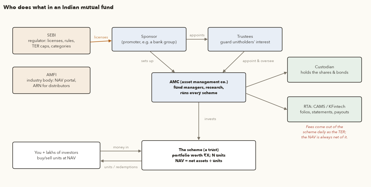
Varsity's practical advice holds: as an investor you mostly care about two things in this structure. Is the sponsor credible and well-capitalised? Who is the fund manager, and how long have they run this scheme? Both are printed in every scheme's factsheet and its SID (Scheme Information Document), the legal offer document.
Open-ended vs closed-ended. Almost all funds you will meet are open-ended: you can buy or redeem units from the fund on any business day at that day's NAV, and the fund has no end date. Closed-ended funds (some fixed-maturity plans, some older ELSS) take money only during the launch and then lock it until a maturity date; their units may trade on the exchange, often at a discount. Interval funds open for redemptions only at set intervals.
3. Units and NAV: what you actually buy
When you invest you receive units, not shares of the companies. The price of one unit is the NAV (net asset value): the fund's net assets divided by the number of units. The AMC computes it at the end of every business day from closing prices.
- Market value of securities
- Everything the fund owns (shares, bonds), valued at today's closing prices, in ₹.
- Cash
- Money in the fund's bank account, in ₹.
- Accrued income
- Interest and dividends earned but not yet received, in ₹.
- Liabilities
- What the fund owes: for example redemptions it must still pay out.
- Accrued expenses
- Fees and costs built up but not yet paid, including today's slice of the TER (part 4).
- Units outstanding
- The total number of units all investors hold.
- NAV
- Net asset value: the value of one unit, in ₹.
- Amount
- The rupees you invest.
- Stamp duty
- 0.005% of the amount (₹5 per ₹1 lakh), taken before units are bought (since 1 Jul 2020).
How it works: add up what the fund owns, subtract what it owes, and divide by the number of units. That is the NAV. When you invest, stamp duty comes off first and the rest buys units at that NAV, usually in fractions (to three decimals). The worked example below does both steps.
A scheme with ₹125 crore of assets
- Securities, cash and accrued interest at today's closing prices: ₹125,00,00,000.
- Liabilities (redemptions payable, today's accrued fee and other expenses): ₹50,00,000.
- Units outstanding: 5,00,00,000.
- NAV = (1,25,00,00,000 − 50,00,000) ÷ 5,00,00,000 = ₹24.90.
- If you invest ₹1,00,000 today, stamp duty of 0.005% (₹5) is deducted first, so you get 99,995 ÷ 24.90 = 4,015.863 units.
Which NAV do you get? Cut-off times
Mutual-fund orders are not priced like share trades. You do not know the price when you place the order: you get the NAV of the day your order (and your money) reaches the fund in time.
| Transaction | Cut-off | NAV you get | Money / units arrive |
|---|---|---|---|
| Buy, equity / debt / hybrid funds | 3:00 pm, with funds credited to the scheme | Same day's closing NAV if the money is realised by the cut-off; otherwise the next business day's | Units within a day or two |
| Buy, liquid and overnight funds | 1:30 pm, with funds credited | NAV of the day before the day the money arrives (these funds accrue interest daily) | Next day |
| Redeem, any scheme | 3:00 pm | Same day's NAV if submitted before cut-off (liquid and overnight funds: the NAV of the day before the next business day, so a Friday request earns the weekend's interest) | SEBI's limit is 3 working days (late payment earns 15% a year interest); most equity funds pay in 2 (T+2), liquid funds next day |
Because the money must reach the fund by the cut-off, a UPI or net-banking payment at 2:58 pm can still miss it. For a long-term SIP this does not matter. It matters when you switch large amounts during a volatile day. ETFs (part 10) are different: they trade on the exchange at live prices and settle T+1 like shares.
AMFI publishes every scheme's NAV on its website each business evening (by 11 pm), and the RTA updates your statement. That NAV already reflects the day's expenses: there is no separate fee bill.
The NFO myth: "₹10 units are cheap"
An NFO (new fund offer) is the launch of a new scheme, usually at ₹10 per unit. Distributors sometimes pitch it as "buying at ₹10 instead of ₹150". That is the same mistake as thinking a low-priced share is cheaper than a high-priced one. A unit's NAV tells you nothing about value: it only reflects when the fund started and how it has done since. What matters is the percentage change.
₹10,000 into a ₹172 NAV vs a ₹239 NAV
- UTI Nifty 50 Index Fund (Direct): NAV ₹171.7458 → ₹159.2891. ₹10,000 buys 58.226 units, worth ₹9,274.70 a year later (−7.25%).
- HDFC Nifty 50 Index Fund (Direct): NAV ₹238.9073 → ₹221.3947. ₹10,000 buys 41.857 units, worth ₹9,266.97 (−7.33%).
- Same index, almost the same outcome. The fund with the lower NAV gave you more units, but each unit moved by the same percentage. The ₹7.73 difference comes from costs and tracking (part 10), not from the NAV level.
A new fund also has no track record, may hold cash while it deploys money, and is often a "theme" launched near the top of that theme's popularity. Unless the NFO offers something genuinely unavailable, an existing fund with a record is usually the better choice.
4. What a fund costs you: TER, exit load, stamp duty, STT
The total expense ratio (TER)
A fund's yearly running cost, as a percentage of its assets, is its TER (total expense ratio). It pays the AMC's management fee, the RTA, custodian, auditors, marketing and, in regular plans, the distributor's commission. You never see a bill. The fund deducts a slice every day before declaring the NAV, so a 1% TER means the NAV grows about 1% a year slower than the portfolio does.
- Net assets
- The fund's total assets minus what it owes, in ₹, on that day.
- TER
- Total expense ratio: the fund's yearly running cost as a percentage of its assets (0.25% for the UTI Nifty 50 index fund's direct plan). Dividing by 365 gives one day's share.
- \(P\)
- The amount you invest at the start, in ₹.
- \(g\)
- The gross yearly return of the fund's portfolio, before costs, as a fraction (11% = 0.11).
- \(t\)
- The TER as a fraction (1% = 0.01).
- \(n\)
- The number of years you stay invested.
- \([\dots]^{n}\)
- The power \(n\): multiply the bracket by itself \(n\) times, once for each year (compounding).
- \(V_n\)
- What your money is worth after \(n\) years, in ₹.
How it works: each day the fund takes 1/365 of the TER out of its assets before it declares the NAV. Over a year that adds up to about the TER. So each year your money grows by \((1+g)\) and then loses the fraction \(t\); after \(n\) years you multiply by that yearly factor \(n\) times. It is "≈" because the fee is really taken daily, not once a year. The ₹10 lakh worked example below plugs in 11%, 0.2% and 1.6%.
Example (illustrative): for the ₹125 crore scheme in part 3, a 1% TER would take 1,25,00,00,000 × 0.01 ÷ 365 ≈ ₹34,247 out of the assets every day, about ₹1.25 crore over a year.
New from 1 Apr 2026. The SEBI (Mutual Funds) Regulations, 2026 replaced the 1996 regulations. They split the old TER into a base expense ratio (BER), which is the AMC's own fee and is capped, plus brokerage and transaction costs (separately capped, and cut sharply) plus statutory and regulatory levies (GST, STT, stamp duty, exchange and SEBI fees) charged at actuals. The caps on the AMC's fee were also lowered, and the extra 0.05% that funds with exit loads were allowed to charge was removed. Fund pages and factsheets now show the BER and the TER separately.
| Open-ended scheme, AUM slab | Max BER, equity-oriented | Max BER, other (debt etc.) |
|---|---|---|
| First ₹500 crore | 2.10% | 1.85% |
| Next ₹250 crore | 1.90% | 1.65% |
| Next ₹1,250 crore | 1.60% | 1.40% |
| Next ₹3,000 crore | 1.50% | 1.25% |
| Next ₹5,000 crore | 1.40% | 1.15% |
| Next ₹40,000 crore | falls by 0.05% for every ₹5,000 crore | |
| Above that | 0.95% | 0.70% |
| Index funds and ETFs | 0.90% (was 1.00%) | |
| Fund of funds: investing in ETFs/index/liquid funds · ≥65% in equity funds · others | 0.90% · 2.10% · 1.85% | |
These are ceilings, applied slab by slab to the fund's assets (AUM, assets under management). Large funds charge far less. On 1 Oct 2026, Groww's scheme pages listed these direct-plan figures: UTI Nifty 50 Index Fund TER 0.25% (BER 0.18%); Parag Parikh Flexi Cap 0.69% (BER 0.53%) on ₹1,47,405 crore of AUM; HDFC Large Cap 1.03% (BER 0.84%). Always check the AMC's own TER page, which is updated whenever the TER changes.
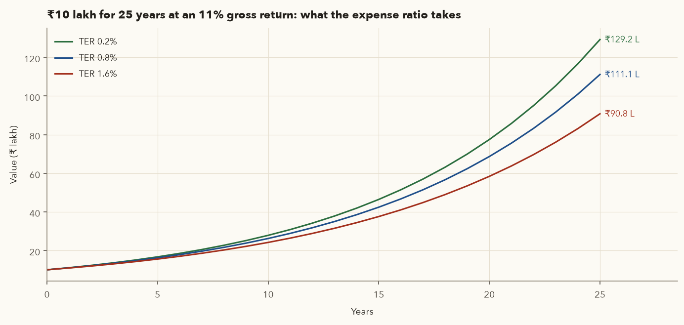
What the expense ratio takes
- With no costs: 10,00,000 × 1.1125 = ₹1,35,85,464.
- TER 0.2%: 10,00,000 × (1.11 × 0.998)25 = ₹1,29,22,246.
- TER 1.6%: 10,00,000 × (1.11 × 0.984)25 = ₹90,77,201.
- Difference: ₹38,45,045, almost four times the money you put in. The fee looks small each year because it is charged on the whole pot, every year, and the pot keeps growing.
Exit loads
An exit load is a fee for redeeming early, deducted from your redemption value and paid back into the scheme (it protects remaining investors from the cost of short-term money). Typical: 1% if redeemed within 12 months for equity funds; nil for index funds and ETFs in many cases; liquid funds have a tiny graded load for the first six days (0.0070% on day 1 down to 0.0045% on day 6, nil from day 7). Redeeming ₹2,50,000 from an equity fund in month 11 costs 1% = ₹2,500. The load applies per unit, by purchase date (first in, first out), so each SIP instalment has its own 12-month clock.
Stamp duty and STT
- Stamp duty: 0.005% of every purchase, SIP instalment, switch-in and STP-in (since 1 Jul 2020; an STP is a systematic transfer from another scheme, part 12). ₹5 per ₹1 lakh. Nothing on redemptions. Transfers of units between demat accounts pay the general 0.015% transfer rate instead.
- STT (Securities Transaction Tax, explained in Chapter 13): 0.001% of the value when you redeem units of an equity-oriented fund with the fund; none on debt-fund redemptions. On an exchange, sales of equity ETFs pay 0.001% STT on the sell side and none on the buy side; gold, silver, debt and international ETFs pay no STT. All ETF trades also pay exchange charges, buy-side stamp duty and, on sell days, the DP charge.
- Brokerage: zero for direct mutual-fund plans on most platforms. ETFs are shares for this purpose: at a discount broker delivery brokerage is ₹0, but the depository (DP) charge, ₹15.34 per stock per sell day at Zerodha, applies.
- Comparing returns without checking the plan. Regular and direct plans of the same fund have different NAVs and returns. Make sure you compare direct with direct.
- Ignoring the TER because "it is only 1%". On a 10–12% gross return, 1% is close to a tenth of your return every year.
- Switching funds inside 12 months. You pay the exit load and, for equity funds, 20% short-term tax (part 13).
- Assuming the TER is the whole cost. Portfolio turnover creates brokerage and impact costs inside the fund. These now appear separately from the BER, but high turnover still costs you something.
5. Direct vs regular plans, on real NAVs
Since 2013 every scheme comes in two versions with the same portfolio:
- Regular plan: bought through a distributor (a bank relationship manager, an agent, many apps). The TER includes a yearly trail commission paid to the distributor for as long as you stay invested.
- Direct plan: bought directly from the AMC, through MF Central, or through a platform that does not take commission (many brokers, the RTA portals). No commission, so a lower TER.
Because the regular plan pays more every day, its NAV falls a little further behind the direct plan every day. The gap shows up only in the NAV, which is why many investors never notice it. The half-yearly Consolidated Account Statement (part 15) does show, in rupees, the commission paid on each regular-plan holding.
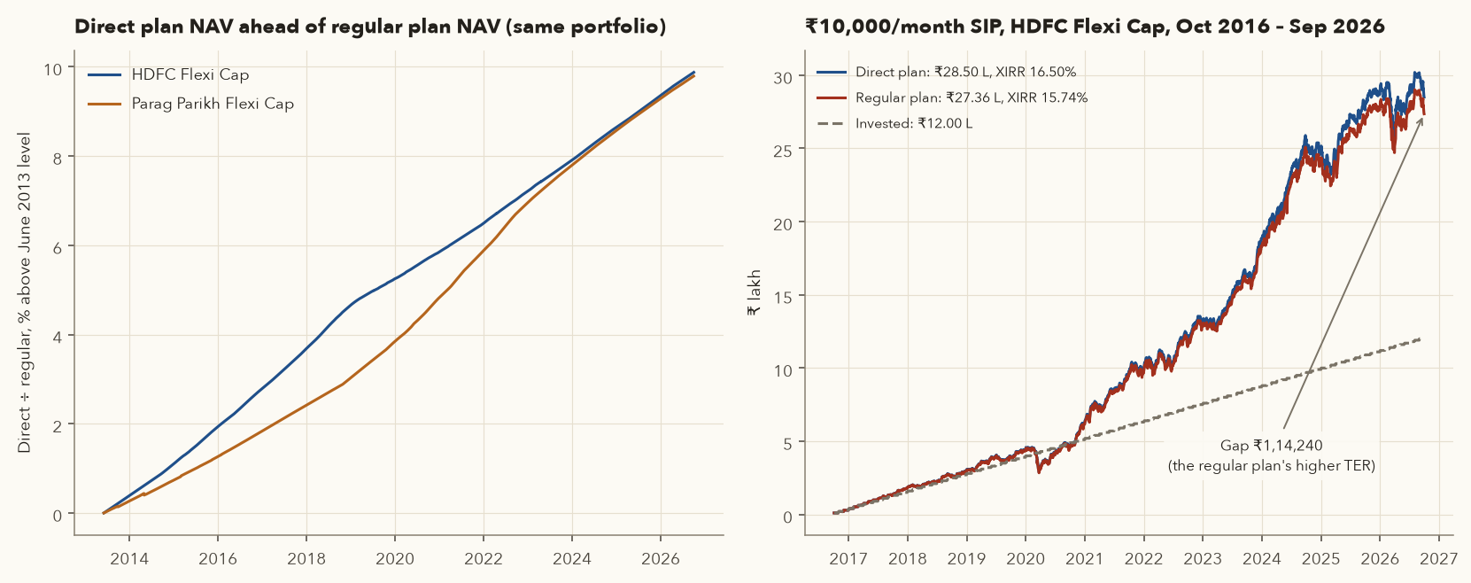
The measured cost of the regular plan
| Fund | 10-yr CAGR direct | 10-yr CAGR regular | Gap a year | 5-yr gap a year |
|---|---|---|---|---|
| HDFC Flexi Cap | 15.52% | 14.72% | 0.80% | 0.76% |
| Parag Parikh Flexi Cap | 16.92% | 16.03% | 0.89% | 0.85% |
A ₹10,000 monthly SIP on the 1st of every month, Oct 2016 – Sep 2026 (120 instalments, ₹12,00,000 invested), valued on 30 Sep 2026:
- HDFC Flexi Cap: direct ₹28,50,357.07 (XIRR 16.50%; XIRR is the yearly return of a series of investments made on different dates, explained in part 12) vs regular ₹27,36,117.28 (XIRR 15.74%). Gap ₹1,14,239.80, 4.18% more money.
- Parag Parikh Flexi Cap: direct ₹28,49,958.71 (XIRR 16.50%) vs regular ₹27,08,794.36 (XIRR 15.55%). Gap ₹1,41,164.36, 5.21% more.
- The gap grows faster than linearly: commission is charged on a pot that keeps growing, and the money not paid as commission compounds for you.
The commission pays for a service. If a distributor genuinely helps you (stops you panic-selling in a crash, keeps your nominations and KYC in order, plans your goals), that behaviour can be worth more than 0.8% a year. If you are doing it yourself, as this course teaches, the direct plan is the same fund for less. An alternative is a SEBI-registered investment adviser (RIA), who charges you a visible fee and must use direct plans. To switch an existing holding from regular to direct, the fund treats it as a redemption and a fresh purchase, so check the exit load and the capital-gains tax first (Chapter 15).
6. SEBI's category map (and the 2025–26 changes)
Before 2017, fund names meant little: two "bluechip" funds could hold completely different things. SEBI's October 2017 circular forced every fund house to fit each scheme into one of about 36 defined categories, with one scheme per category (index funds, ETFs and FoFs excepted). The definitions are about what the fund must hold. Market-cap buckets use AMFI's half-yearly list: large cap = the 100 largest listed companies by full market cap, mid cap = 101st–250th, small cap = 251st onwards (Chapter 1).
Equity schemes
| Category | Rule (share of assets) | What it means for you |
|---|---|---|
| Large cap | ≥ 80% in large caps | Closest to the index; hardest category in which to beat the benchmark |
| Large & mid cap | ≥ 35% large and ≥ 35% mid | More growth, more volatility |
| Multi cap | ≥ 75% equity, with ≥ 25% each in large, mid and small | Forced small-cap exposure even in bad times |
| Flexi cap | ≥ 65% equity, any mix of sizes | Manager decides; a popular single "core" fund |
| Mid cap / Small cap | ≥ 65% in mid / small caps | Higher return potential and much deeper falls; small caps can be hard to sell |
| Value / Contra | ≥ 65% equity, value or contrarian style | Style can lag for years. From 2026 a fund house may offer both, if their portfolios overlap by no more than 50% |
| Focused | ≥ 65% equity, at most 30 stocks | Concentrated: more manager risk |
| Dividend yield | ≥ 65% in dividend-yielding stocks | A style, not an income guarantee |
| Sectoral / thematic | ≥ 80% in one sector or theme | Satellite-only. From 2026, overlap with the house's other equity schemes (except large cap) is capped at 50% |
| ELSS (equity-linked saving scheme) | ≥ 80% equity, 3-year lock-in | Tax deduction only under the old tax regime (old s.80C); ch15 discusses whether it still fits |
Debt schemes (16 categories)
Debt funds are defined either by duration (how sensitive they are to interest rates, part 8) or by what they hold (credit quality, issuer type). Overnight (1-day securities), liquid (maturity up to 91 days), ultra-short (Macaulay duration 3–6 months), low duration (6–12 months), money market (maturity up to 1 year), short (1–3 years), medium (3–4 years), medium to long (4–7 years), long (over 7 years) and dynamic bond (any) are duration categories. By holdings: corporate bond (≥ 80% in AA+ and above), credit risk (≥ 65% below AA+, i.e. riskier borrowers), banking & PSU (≥ 80% in banks, PSUs and public financial institutions), gilt (≥ 80% government securities), gilt with 10-year constant duration, and floater (≥ 65% floating-rate bonds).
Hybrid schemes
| Category | Equity share | Note |
|---|---|---|
| Conservative hybrid | 10–25% | Mostly debt |
| Balanced hybrid / Aggressive hybrid | 40–60% / 65–80% | A house may offer one of the two |
| Dynamic asset allocation (balanced advantage) | 0–100%, managed by a model | Many keep ≥ 65% "gross" equity using hedged positions, which matters for tax |
| Multi-asset allocation | ≥ 3 asset classes, ≥ 10% each | Often equity + debt + gold/silver |
| Arbitrage | ≥ 65% in hedged cash-futures arbitrage | Debt-like returns, equity tax (part 11) |
| Equity savings | ≥ 65% equity incl. hedged, ≥ 10% debt | Low-volatility equity tax structure |
Others, and what changed in 2025–26
- Index funds and ETFs (≥ 95% in the index's constituents) and fund of funds (FoF: ≥ 95% in other funds, domestic or overseas).
- Life cycle funds (new, Feb 2026). SEBI's 26 Feb 2026 circular on categorisation (which superseded drafts of Oct and Nov 2025) created life cycle funds: target-date funds with a stated maturity year (5 to 30 years, in 5-year steps, the year in the name, e.g. "…2045"), following a glide path that moves from mostly equity (65–95% when far away) to mostly debt near the end. They carry a steep exit load (3% in year 1, 2% in year 2, 1% in year 3) to discourage early exits. The same circular stopped fresh money into solution-oriented (retirement and children's) funds; on 20 Mar 2026 SEBI allowed fund houses to keep those schemes, with limits on which life cycle tenures they may then launch. If you hold such a scheme, check its latest notice.
- Residual money in equity schemes may now go into gold, silver and InvITs as well as debt, and REITs count as equity for mutual funds from 1 Jan 2026 (InvITs remain hybrid).
- Specialised Investment Funds (SIF), from 1 Apr 2025: a new product inside the mutual-fund structure that can run long-short equity, long-short debt and similar strategies (unhedged shorts up to 25% of assets). Minimum ₹10 lakh per investor (PAN) across a fund house's SIF strategies. Not a beginner product.
Two flexi-cap funds can still be very different (part 14 shows overlap as low as 30%). A category tells you the rules the manager must follow, and therefore the benchmark to judge them against. It does not tell you whether the fund is good.
7. Reading a factsheet and the riskometer
Every fund house publishes a monthly factsheet per scheme (and the full portfolio by the 10th of the next month). Varsity spends several chapters on it; here is what each item tells you, and the formula behind the risk numbers.
| Item | What it is | How to use it |
|---|---|---|
| Investment objective, benchmark | What the fund promises to do, and the TRI (total return index, dividends reinvested) it is measured against | Compare the fund only with its TRI, never with the price index |
| AUM, launch date, fund manager and tenure | Size and history | Very small funds can close or merge; very large small-cap funds struggle to deploy money |
| TER (BER), exit load | Costs (part 4) | Direct plan's TER is the one that applies to you |
| Portfolio, sector weights, top 10 | What you actually own | Check overlap with your other funds (part 14) |
| Portfolio turnover | Value of buying or selling in a year ÷ average assets | Groww listed ICICI Pru Large Cap at 51% and SBI Large Cap at 8% (Oct 2026): very different styles |
| Standard deviation | Annualised volatility of returns | Higher = bumpier ride (Chapter 11) |
| Beta | Sensitivity to the benchmark: 1.1 means about 1.1% move for 1% in the index | Beta above 1 in a "defensive" fund is a warning |
| Sharpe ratio | Return above the risk-free rate per unit of volatility | Compare only within a category, over the same period |
| Alpha | Return above what the beta would predict | Often quoted over short periods; check rolling returns instead (part 9) |
| Debt: YTM, average maturity, Macaulay and modified duration, credit ratings | Expected yield if held to maturity, interest-rate sensitivity, credit quality | Part 8 |
- \(R_{fund}\)
- The fund's annualised return over the period (usually 3 years on a factsheet), in % a year.
- \(R_{bench}\)
- The benchmark TRI's annualised return over the same period.
- \(R_f\)
- The risk-free rate: what a near-riskless investment paid over the period, such as a short-term government bill or overnight money-market rate. The factsheet footnote says which rate it used.
- \(\sigma_{fund}\)
- The fund's annualised standard deviation (volatility) of returns, in %.
- \(r_{fund},\ r_{bench}\)
- Lower-case \(r\): the individual periodic returns (daily, weekly or monthly) of the fund and the benchmark, not the annual figure.
- \(\operatorname{Cov}\)
- Covariance: how much the two returns move together, scaled by how much each moves.
- \(\operatorname{Var}\)
- Variance: the standard deviation squared, a measure of how much the benchmark's returns swing.
- Sharpe
- Extra return over the risk-free rate earned for each 1% of volatility. Higher is better.
- \(\beta\)
- Beta: how much the fund tends to move for a 1% move in the benchmark.
- \(\alpha\)
- Alpha, in % a year: the return above what the fund's beta alone would have earned.
- Sharpe: take the fund's return, subtract the risk-free rate, and divide by the fund's volatility.
- Beta: from the periodic returns, divide the covariance of fund and benchmark by the benchmark's variance. This is the slope of a line fitted through (benchmark return, fund return) points.
- Alpha: the bracket is the return you would "expect" for that beta: the risk-free rate plus beta times the benchmark's extra return. Alpha is what the fund earned above that.
Example (illustrative round numbers): fund 12% a year, benchmark 11%, risk-free 6.5%, fund volatility 15%, beta 0.9. Sharpe = (12 − 6.5) ÷ 15 = 0.37. Expected return for beta 0.9 = 6.5 + 0.9 × (11 − 6.5) = 10.55%, so alpha = 12 − 10.55 = 1.45% a year.
Riskometer. Each scheme carries a SEBI-prescribed riskometer with six levels: Low, Low to Moderate, Moderate, Moderately High, High, Very High. The AMC assesses it monthly from the portfolio (volatility, market cap, liquidity, credit and duration) and must also show the benchmark's level. Almost every equity fund, index funds included, sits at High or Very High. It is a useful sanity check, not a forecast. Debt funds also show a Potential Risk Class (PRC) matrix: credit risk A (lowest) to C, against interest-rate risk I (lowest) to III. A fund in cell A-I is the most conservative; C-III can lose money from both defaults and rate rises.
8. Debt funds: interest-rate, credit and liquidity risk
A debt fund owns loans: government securities (G-secs; T-bills if under a year), state development loans, corporate bonds, commercial paper (short-term company IOUs) and bank certificates of deposit. Its NAV moves for three reasons: interest accrues every day (the steady part), bond prices change when market yields change, and borrowers can default. The YTM (yield to maturity) is the return the portfolio would earn if every bond were held to maturity and paid in full; after costs, it is the best rough guide to a debt fund's future return over its duration.
Interest-rate risk and duration
When market yields rise, existing bonds with lower coupons become less attractive, so their prices fall until their yield matches the market. The longer the bond, the bigger the fall. Macaulay duration is the weighted average time (in years) until you receive the bond's cash flows. Modified duration converts that into price sensitivity: roughly the percentage fall in price for a 1 percentage point rise in yield.
- \(t\)
- When a cash flow arrives, in years from today: 0.5, 1, 1.5 … for half-yearly coupons.
- \(CF_t\)
- The cash flow at time \(t\), in ₹: a coupon, plus the face value at maturity.
- \(y\)
- The bond's yield to maturity per year, as a fraction (6.75% = 0.0675). \(y/2\) is the half-yearly rate.
- \((1+y/2)^{2t}\)
- Discounting: a cash flow \(2t\) half-years away is divided by \((1+y/2)\) once for each half-year, giving its value today.
- \(\sum_t\)
- "Add up over every cash flow" (capital sigma means "sum").
- \(P\)
- The bond's price today: the sum of all discounted cash flows.
- \(D_{mac}\)
- Macaulay duration, in years: the average time until you are paid, each payment weighted by its share of today's price.
- \(D_{mod}\)
- Modified duration: roughly the % fall in price for a 1 percentage point rise in yield.
- \(\Delta y,\ \Delta P\)
- "Change in" the yield (in percentage points) and in the price. \(\Delta P / P\) is the % price change.
- Discount each coupon and the final repayment to today's value. Their total is the price \(P\).
- Multiply each discounted amount by its time \(t\), add these up, and divide by \(P\). That is \(D_{mac}\).
- Divide by \(1 + y/2\) to get \(D_{mod}\).
- Price change ≈ minus \(D_{mod}\) times the change in yield. The minus sign says prices fall when yields rise.
For a debt fund over a short period: total return ≈ yield accrued (carry) − \(D_{mod} \times \Delta y\). "Carry" is the interest earned over the period: the yield × days ÷ 365. The gilt-fund example below uses exactly this.
Yields rose 0.43 points. What should the NAV have done?
- The 10-year G-sec yield went from 6.75% (30 Jun 2026) to 7.18% (30 Sep 2026): \(\Delta y = +0.43\) percentage points.
- The fund holds about 10-year G-secs. For a 10-year bond priced near par at 6.75% with half-yearly coupons, \(D_{mac}\) = 7.43 years and \(D_{mod} = 7.43 / 1.03375 = 7.19\).
- Price effect ≈ −7.19 × 0.43% = −3.09% (the exact repricing gives −3.03%; the gap is convexity: the price–yield curve bends, so the straight-line duration estimate slightly overstates falls and understates rises).
- Carry: 92 days of 6.75% yield ≈ 6.75% × 92/365 = +1.70%.
- Predicted change ≈ −3.09% + 1.70% = −1.39%. Actual NAV: ₹26.6570 → ₹26.3587, −1.12%. Close, given that the fund's exact holdings and duration differ a little from our one-bond model and costs are ignored.
The same thing happened in the 2022 rate-hike scare: the yield rose from 6.84% (31 Mar) to 7.42% (31 May 2022) and the fund's NAV fell 2.78%. Over the full year to 30 Sep 2026, as yields rose from 6.57% to 7.18%, this gilt fund returned only 3.70%, less than a liquid fund (6.46%). A "safe" government-bond fund carries no default risk but a lot of interest-rate risk.
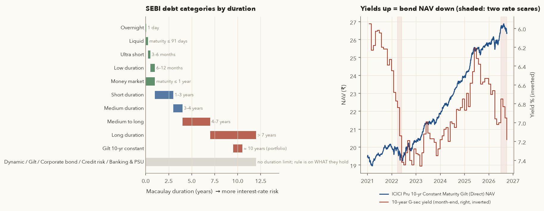
Rule of thumb: hold a debt fund for at least as long as its Macaulay duration; Varsity's stricter version is its average maturity. Over that period, the higher yield earned after a rise roughly makes up for the price fall. Money you need in 6 months belongs in a liquid or overnight fund, not a gilt fund.
Credit risk and liquidity risk: the Franklin Templeton wind-up
Credit risk is the chance that a borrower pays late or not at all. Liquidity risk is the chance that the fund cannot sell bonds quickly enough at a fair price to pay redemptions. In India's corporate-bond market, where many bonds rarely trade, the two often arrive together.
Six debt funds closed overnight
- Franklin Templeton's debt funds had chased extra yield in lower-rated, unlisted and illiquid papers. Defaults and downgrades (Vodafone Idea, Yes Bank and others) began to hit NAVs in early 2020: the Franklin India Credit Risk Fund NAV fell from ₹20.0370 (10 Jan 2020) to ₹18.1028 (30 Apr 2020), −9.65%, in a category sold as "stable income".
- When the Covid crash triggered heavy redemptions and the bond market froze, the trustees wound up six schemes (Ultra Short Bond, Low Duration, Short Term Income Plan, Income Opportunities, Credit Risk, Dynamic Accrual), about ₹25,000 crore. Redemptions stopped immediately.
- Investors were repaid in instalments as the bonds matured or were sold, a process that ran for years through court cases (including in the Supreme Court). Franklin reports ₹27,548.21 crore distributed, 109.25% of the 23 Apr 2020 AUM.
- So most investors eventually got their money back with some return, but they could not use it when they needed it, and the "ultra short" fund many treated as a savings account was locked too.
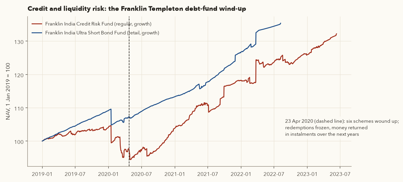
After this, SEBI tightened liquidity rules: most open-ended debt funds must now keep a minimum share of their assets in liquid securities. SEBI had already allowed segregated portfolios ("side-pockets") since late 2018: when a bond defaults, the fund can split it off into a separate portfolio so that new money does not subsidise old losses and existing holders keep their claim on any recovery. You can see such units in the Franklin scheme list ("Segregated Portfolio 1 – 8.25% Vodafone Idea"). Lessons: in debt funds, chase quality and liquidity, not the highest YTM; avoid credit-risk funds unless you understand every large holding; check concentration (a single issuer above 5–10% is a red flag); prefer large, plain categories (liquid, money market, short duration, corporate bond, banking & PSU, gilt) for core money.
9. Active vs passive: what the data says
An active fund pays a manager to pick securities and try to beat the benchmark. A passive fund (index fund or ETF) simply buys the benchmark's stocks in the benchmark's weights and accepts the index return minus a small cost. The question is not "can a manager beat the index?" (some do) but "can you pick, in advance, the ones that will, after fees?"
The SPIVA scorecard
S&P Dow Jones Indices publishes the SPIVA India scorecard twice a year. It counts every fund that existed at the start of each period, including those that were merged or closed, and compares their returns with a benchmark. In the Year-End 2025 report (the latest available on 2 Oct 2026), active Indian large-cap funds underperformed their benchmark at rates of 75.0% over 1 year, 74.2% over 3, 84.4% over 5 and 76.3% over 10 years. In 2025 alone, 69.2% of ELSS funds lagged their benchmark. Active mid- and small-cap funds had their best relative year since 2014 in 2025, with a majority beating their benchmark, but over 10 years a majority in every category lagged.
Our own mini-scorecard, from NAVs
We repeated the exercise with data anyone can download: every large-cap direct-plan scheme in AMFI's list (via mfapi), alive or dead, against the Nifty 100 TRI (the benchmark most of them use) and against a real index fund (UTI Nifty 50 Index Fund, Direct). A fund that was merged away during the period counts as "did not survive".
| Period to 30 Sep 2026 | Funds at start | Merged / closed | Beat Nifty 100 TRI | Nifty 100 TRI | Index fund (N50) | Median survivor |
|---|---|---|---|---|---|---|
| 3 years | 29 | 0 | 21 (72.4%) | 7.81% | 5.83% | 9.15% |
| 5 years | 32 | 6 | 19 (59.4%) | 7.06% | 6.14% | 8.41% |
| 10 years | 27 | 6 | 11 (40.7%) | 11.68% | 11.18% | 11.78% |
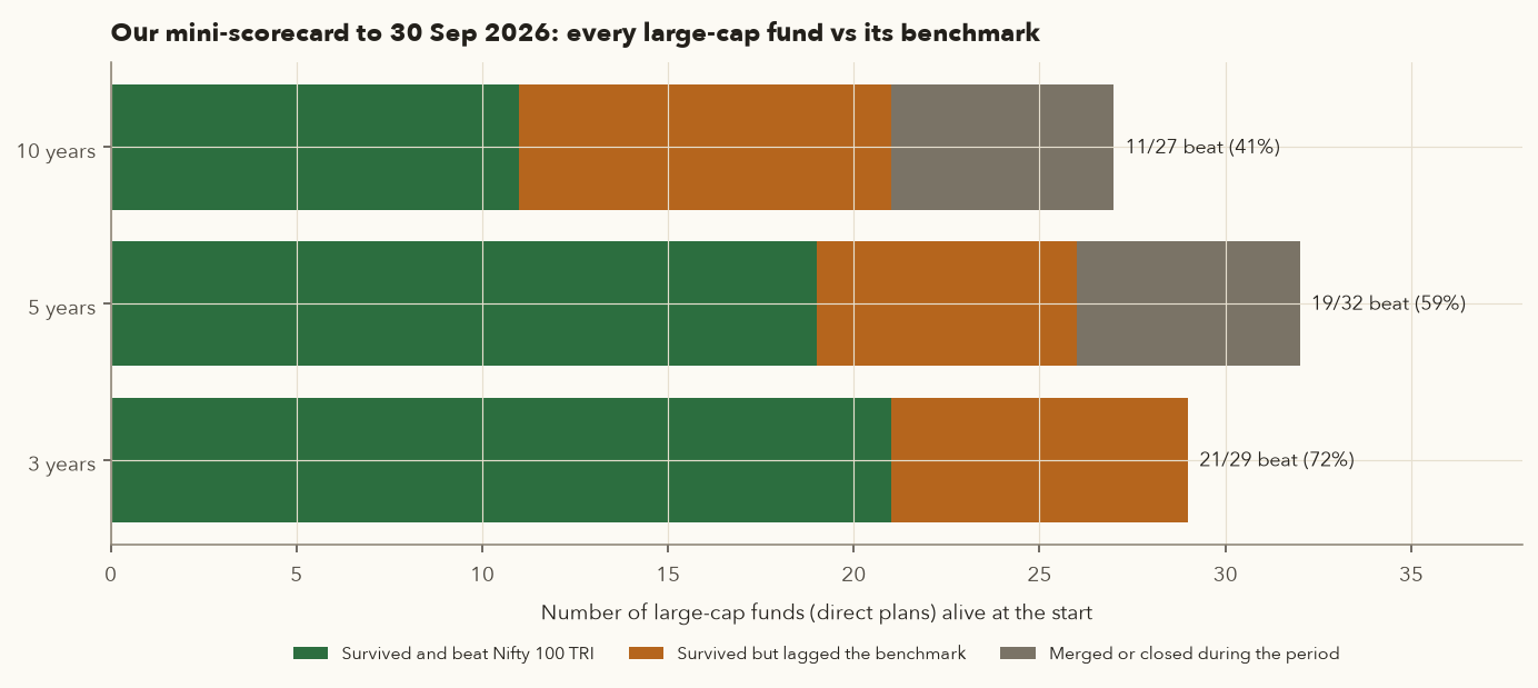
This is an honest, mixed picture, and kinder to active funds than SPIVA's. Three reasons. First, the recent period was unusually good for active large-cap funds against the Nifty 50 and Nifty 100: the very largest stocks lagged, and funds holding more mid-sized companies benefited. Second, SPIVA measures against S&P's own India indices and uses its own fund database, and the choice of benchmark alone can swing the answer (quiz Q6 shows how much). Third, we used direct plans, the cheapest version; most investors held regular plans, which are 0.6–0.9% a year more expensive, so with regular plans fewer funds would clear the bar. The longer the period, the worse active funds look: over 10 years the median surviving fund (11.78%) only matched the benchmark, while the index fund (11.18%) lost just its cost.
Rolling returns: judging four big names
A single start and end date ("point-to-point") can flatter or damn any fund. Rolling returns compute the CAGR for every possible start date: the 5-year return from every trading day to the day five years later. Varsity recommends looking at the average, minimum, maximum and how often the fund beat its benchmark.
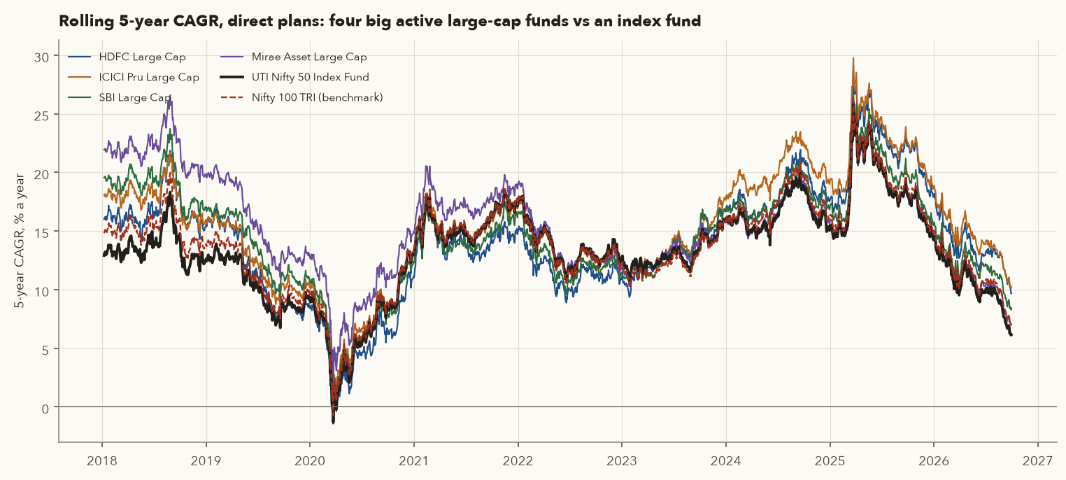
How often each fund beat an index fund
| Direct plan | 10-yr CAGR | 5-yr periods beating the index fund | beating Nifty 100 TRI | Worst 5-yr CAGR |
|---|---|---|---|---|
| ICICI Pru Large Cap | 13.15% | 83.7% | 83.0% | 0.01% |
| Mirae Asset Large Cap | 12.35% | 84.4% | 65.0% | 2.06% |
| HDFC Large Cap | 11.98% | 60.0% | 58.9% | −1.45% |
| SBI Large Cap | 11.64% | 66.9% | 68.7% | −0.24% |
| UTI Nifty 50 Index Fund | 11.18% | — | — | −1.32% |
These four did beat the index fund more often than not. But be careful what you conclude. They are four of the largest surviving funds, chosen today, with hindsight: that is survivorship bias (Chapter 12). In 2016 nobody knew that L&T, BNP Paribas, IDBI and three others would disappear, and the 10-year scorecard shows that a randomly chosen large-cap fund was more likely than not to lag. Mirae's 5-year lead over the index fund shrank from about 9 points in early 2018 to 0.9 points by Sep 2026.
For the large-cap part of a core portfolio, an index fund is the default: low cost, no manager risk, and, because it lags its index only by its small cost, it is unlikely to end up in the bottom quarter of its category over long periods. Active funds have a better case in mid- and small-caps and flexi-cap, where markets are less efficient, but there you need the discipline to judge them on rolling returns against the right TRI, at least every year, and to accept periods of lagging. Many investors split the difference: an index fund as the core and one active fund beside it.
10. Index funds vs ETFs: plumbing, premiums and tracking
Both track an index. The difference is how you buy and sell.
- An index fund is an ordinary open-ended mutual fund: you buy from the AMC at the day's NAV, any rupee amount, SIP-friendly, no demat account needed.
- An ETF (exchange-traded fund) is a fund whose units are listed on the exchange: you buy from other investors through your broker at the live market price, in whole units, into your demat account, like a share. NIFTYBEES, GOLDBEES, LIQUIDBEES and SILVERBEES are ETFs.
How an ETF stays near its NAV: creation and redemption
New ETF units are not created by the exchange. Big players called authorised participants or market makers deliver a basket of the index stocks (or cash) to the AMC in large blocks called creation units and receive new ETF units, or do the reverse to redeem. If the ETF trades above the value of its basket, they create units and sell them; if below, they buy units and redeem them. This arbitrage keeps the market price close to NAV, as long as the market makers can do it cheaply. SEBI allows direct creation or redemption with the AMC only for market makers and for orders above about ₹25 crore; ordinary investors trade on the exchange. If an ETF trades at a significant discount or has no quotes for several days, the AMC must let ordinary investors redeem directly at NAV (the triggers are in each SID).
During market hours the AMC and exchange publish an iNAV (indicative NAV): an estimate of the current value of one unit, updated through the day. Before you place an ETF order, compare the price with the iNAV, and use a limit order rather than a market order.
- Market price
- The ETF's price on the exchange (the closing price, or the live price during the day), in ₹.
- NAV
- The value of the ETF's holdings per unit, in ₹ (or the iNAV during market hours).
- Premium
- How much more than its NAV you pay for a unit, as a fraction (×100 for %). Negative means a discount.
- \(R_{fund},\ R_{index\ TRI}\)
- The fund's CAGR and the CAGR of the index it tracks (the total return index, with dividends reinvested) over the same period, in % a year.
- TD
- Tracking difference, in % a year: return lost (negative) or gained against the index.
- \(r_{fund,t},\ r_{index,t}\)
- The fund's and the index's return on one day \(t\).
- stdev
- The standard deviation: how much the daily gaps vary around their average.
- \(\sqrt{252}\)
- The square root of 252, the number of trading days in a year. Multiplying a daily standard deviation by it turns it into a yearly one.
- TE
- Tracking error, in % a year: how unevenly the fund follows the index.
- Premium: subtract the NAV from the price and divide by the NAV.
- Tracking difference: compute both CAGRs over the same dates and subtract. This is the cost you actually paid.
- Tracking error: for every day, subtract the index's return from the fund's. Take the standard deviation of that column of gaps and multiply by \(\sqrt{252}\).
Example (5 years to 30 Sep 2026, table below): NIFTYBEES's NAV grew 6.331% a year, the Nifty 50 TRI 6.375%, so TD = 6.331 − 6.375 = −0.044% a year. The MON100 example below works out a premium.
When the plumbing breaks: real premiums
Paying ₹1.22 for ₹1 of US stocks
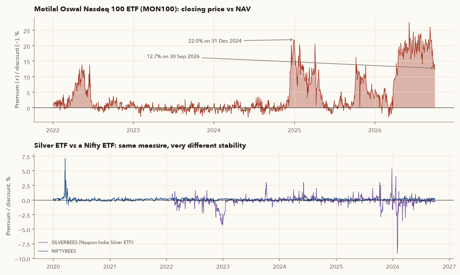
- Indian funds have an industry-wide cap on overseas investment (US$7 billion, plus US$1 billion for overseas ETFs, with per-fund-house limits). When the cap is reached, the AMC cannot create new MON100 units, so the arbitrage that holds the price near NAV stops working.
- On 31 Dec 2024 MON100 closed at ₹214.21 while its NAV was ₹175.6505: a premium of \((214.21 - 175.6505) / 175.6505 = \) 21.95%.
- By 30 Sep 2026 the NAV had risen 62.15% (to ₹284.8257) but the price only 49.89% (to ₹321.08), because the premium shrank to 12.73%. A buyer at the peak premium lost about 12 percentage points of the Nasdaq's gain to the premium.
- The obvious escape, the same AMC's Nasdaq 100 fund of funds, did not help: it holds MON100 units valued at their market price, so its NAV carried the same premium (FoF NAV ÷ ETF price stayed at 0.212–0.211). The FoF returned 49.13% over the same period.
- Across 1,167 trading days from Jan 2022, MON100's closing price was more than 1% away from NAV on 59.8% of days; the maximum premium was 27.67% (5 Jun 2026).
Premiums, discounts, and a NAV that lags
- In October 2025 a physical silver shortage in India made it hard for market makers to source silver to create units. Silver ETFs traded above their NAV; news reports cited intraday gaps of 5–12% against iNAV, and several AMCs (Tata, Axis, Kotak, UTI, SBI, ICICI Pru) paused lump-sum subscriptions to their silver FoFs. On closing prices, SILVERBEES's biggest gap that month was 3.02% (9 Oct 2025: price ₹156.16, NAV ₹151.579).
- The opposite happened on 30 Jan 2026, when silver crashed: SILVERBEES closed at ₹286.48 against a NAV of ₹315.607, an apparent 9.23% discount. By 2 Feb the NAV was ₹237.858 and the price ₹219.94. The price had already reflected the fall; the NAV, based on an earlier silver price, had not. A discount can mean the NAV is stale, not that the ETF is cheap.
- For comparison, NIFTYBEES (from Jan 2020) was more than 1% from NAV on just 0.8% of days, with a median premium of 0.064%. Its one big gap (7.12% on 18 Mar 2020) came in the Covid crash.
Tracking difference and tracking error
These two are often confused. Tracking difference is how much return you actually lost (or, rarely, gained) against the index over a period: mostly the TER plus cash drag and trading costs. Tracking error is how unevenly the fund follows the index day to day: the standard deviation of the daily return gap. A fund can have a tiny tracking error and still a large tracking difference (it follows the index closely but leaks a fixed fee). For a long-term investor, tracking difference is what costs money; tracking error tells you about the quality of execution.
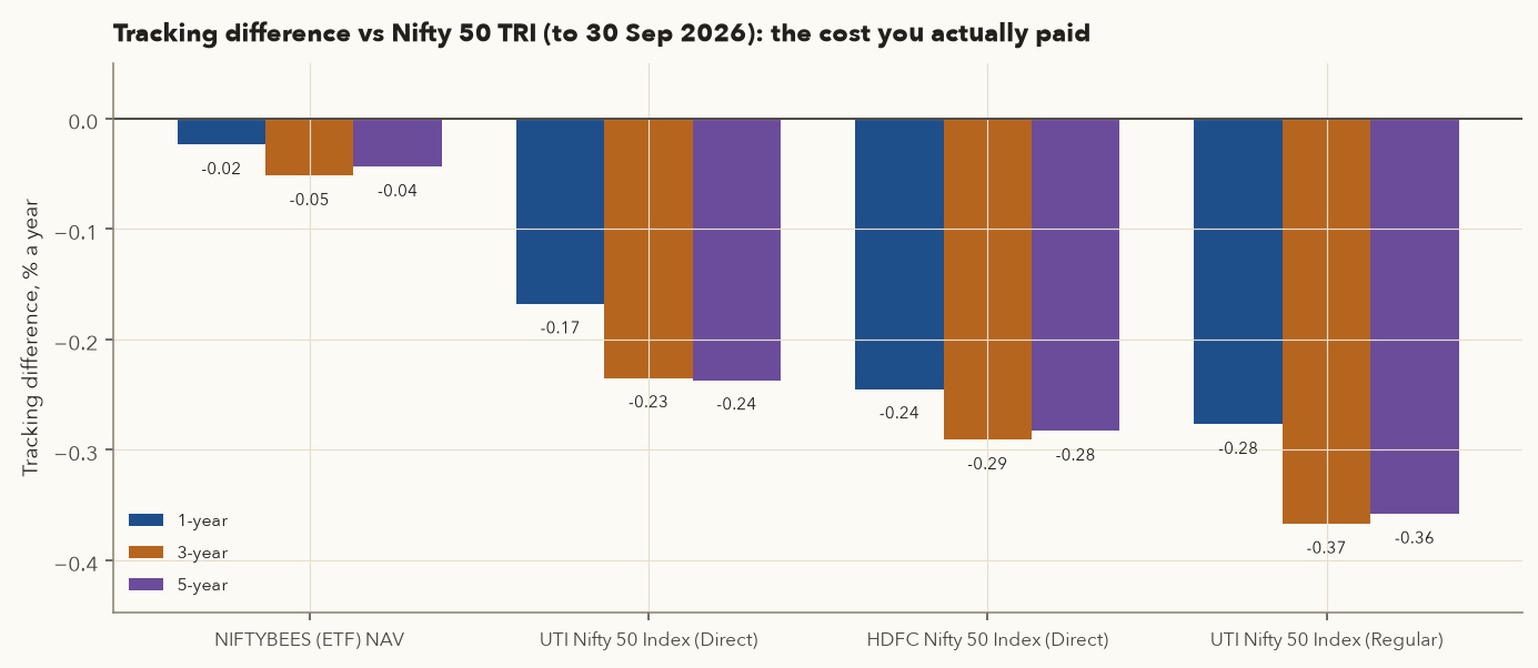
| Nifty 50 tracker (to 30 Sep 2026) | 5-yr CAGR | Tracking difference / yr | Tracking error (5 yr) |
|---|---|---|---|
| Nifty 50 TRI (the target) | 6.375% | — | — |
| NIFTYBEES (ETF), NAV | 6.331% | −0.044% | 0.031% |
| UTI Nifty 50 Index Fund, Direct | 6.139% | −0.237% | 0.032% |
| HDFC Nifty 50 Index Fund, Direct | 6.092% | −0.283% | 0.036% |
| UTI Nifty 50 Index Fund, Regular | 6.017% | −0.358% | 0.034% |
Remember that an ETF investor's real return is based on the prices paid and received, not the NAV, so add half the bid-ask spread (the gap between the best price buyers are bidding and the best price sellers are asking) on each side, any premium you paid, brokerage, the DP charge and STT. For a liquid ETF like NIFTYBEES these are tiny; for an illiquid sector or international ETF they can exceed a year's TER.
Index fund or ETF?
| Index fund | ETF | |
|---|---|---|
| Price you get | NAV after the cut-off; you cannot pay a premium | Live market price; can be above or below NAV |
| Cost | TER usually 0.1–0.3% (direct) | TER often lower (0.03–0.1% for big Nifty ETFs) + brokerage/DP charge + spread |
| Account | None needed (statement of account), or demat | Demat and trading account required |
| SIP | Automatic, any amount | Possible through some brokers, in whole units |
| Liquidity risk | None to you: the fund redeems | Depends on market makers; check volume and spread |
| Margin use | Can be pledged at some brokers | Commonly accepted as collateral for F&O margin |
A simple rule: for a monthly SIP and no wish to watch prices, use a direct index fund. For larger lump sums, tax harvesting (Chapter 13 used NIFTYBEES) or collateral, a large, liquid ETF is cheaper, provided you check the iNAV and use limit orders.
11. Gold, silver, international, REITs and cash parking
Gold and silver
- Gold ETFs (e.g. GOLDBEES) hold physical gold of 99.5% purity in a vault, valued off the international price converted to rupees plus import costs. Each unit is a fraction of a gram. GOLDBEES's NAV grew 27.16% in the year to 30 Sep 2026 and 24.98% a year over five years. Chapter 1 showed gold beating the Nifty over the last decade; that is not a promise for the next.
- Gold FoFs hold units of a gold ETF, so you can SIP any amount without a demat account, for an extra layer of TER. HDFC Gold ETF FoF (Direct) returned 26.46% (1 year) and 25.08% (5 years a year), close to the ETF.
- Sovereign Gold Bonds (SGBs), government bonds linked to the gold price plus 2.5% interest, are no longer issued: the last tranche was in February 2024 and none has been announced for 2025-26 or 2026-27. Existing bonds can be bought on the exchange or redeemed early with the RBI after five years. Budget 2026 limited the capital-gains exemption at redemption to original subscribers who hold until maturity (Chapter 15).
- Silver ETFs and FoFs (launched from 2022) work the same way and are far more volatile: SILVERBEES's NAV rose 53.72% in the year to Sep 2026, yet fell by about a third between 29 Jan and 2 Feb 2026. Treat silver as a small satellite holding, if at all.
International funds
You can get foreign exposure through international FoFs and ETFs (US, Nasdaq, global) or directly through the Liberalised Remittance Scheme (Chapter 13). Domestic funds' overseas investment is capped industry-wide (part 10), so many international funds stop taking lump sums or SIPs from time to time, and ETFs can trade at large premiums. Your return includes the rupee's fall against the dollar, which has helped Indian investors historically.
REITs and InvITs, briefly
REITs (real estate investment trusts, mainly office parks and malls) and InvITs (infrastructure trusts: roads, power lines, pipelines) are listed trusts that must pay out most of their cash flow. They trade like shares, now in lots of one unit. Distributions come in parts (interest, dividend, rent, repayment of debt) that are taxed differently: interest and rent at your slab rate, the dividend part often tax-free, depending on the trust. The trust's yearly tax statement shows the split. This course does not cover REIT tax further; ask a CA if you hold them. Since 1 Jan 2026 mutual funds treat REITs as equity for their portfolio rules; this does not change your own tax rules.
Cash parking: liquid funds, liquid ETFs and arbitrage funds
Money you need soon, or trading cash waiting for a setup, should not sit in an equity fund. Three choices:
| Instrument (direct plans) | 1-yr return to 30 Sep 2026 | 3-yr CAGR | Notes |
|---|---|---|---|
| Liquid fund (HDFC Liquid, Direct) | 6.46% | 6.92% | Securities up to 91 days; redemption next day; "instant redemption" up to ₹50,000 or 90% of holdings, whichever is lower; taxed at slab |
| Liquid ETF, growth version (Nippon India Nifty 1D Rate Liquid ETF) | 4.72% | — | Overnight (1-day) lending; trades on exchange, T+1; LIQUIDBEES is the older version that credits daily dividends as extra units, so its price stays near ₹1,000 |
| Arbitrage fund (Kotak Arbitrage, Direct) | 6.78% | 7.46% | Buys shares and sells futures on them, capturing the gap (Chapter 9); taxed as equity, so better post-tax in high slabs; returns shrink when futures premiums are thin; usually a 0.25% exit load for 15–30 days |
The liquid fund and the overnight liquid ETF lend for different terms (up to 91 days versus overnight), so their yields differ; neither is a bank deposit. As Varsity puts it, a liquid fund is not a savings account: it carries a small credit risk, which is why the category's quality matters.
Which of the three wins after tax depends on your slab and how long you hold. Chapter 15, part 14 works it out on real NAVs.
12. SIPs, rupee-cost averaging, XIRR, STP and SWP
A SIP (systematic investment plan) is a standing instruction to invest a fixed amount on a fixed date every month (or week, or quarter). The amount is debited by auto-debit (NACH/UPI mandate) and units are bought at that day's NAV. A SIP is a habit-making device: it turns investing into a bill you pay yourself first, and it removes the temptation to time the market.
Rupee-cost averaging: what is true
Because you invest the same rupees each month, you automatically buy more units when the NAV is low and fewer when it is high. Your average cost per unit is therefore the harmonic mean of the NAVs you paid, which is always at or below their simple average.
- \(A\)
- The fixed amount of each instalment, in ₹ (ignoring the tiny stamp duty).
- \(n\)
- The number of instalments so far.
- \(i\)
- Which instalment: 1 for the first, 2 for the second, up to \(n\).
- \(\text{NAV}_i\)
- The NAV at which instalment \(i\) was bought, in ₹.
- \(A/\text{NAV}_i\)
- Units bought by instalment \(i\).
- \(\sum_{i=1}^{n}\)
- "Add up for every instalment from 1 to \(n\)."
- \(n \cdot A\)
- The total rupees invested.
- \(\frac{1}{n}\sum_i \text{NAV}_i\)
- The simple average of the NAVs you paid.
- Average cost = total rupees ÷ total units. Total units is the sum of each instalment's units.
- The \(A\) cancels top and bottom, leaving \(n\) divided by the sum of \(1/\text{NAV}\): the "harmonic mean" of the NAVs.
- The ≤ sign says this is never above the simple average NAV. The cheap months buy more units, so they count for more. The UTI SIP below shows ₹95.22 against ₹110.29.
One real SIP, step by step
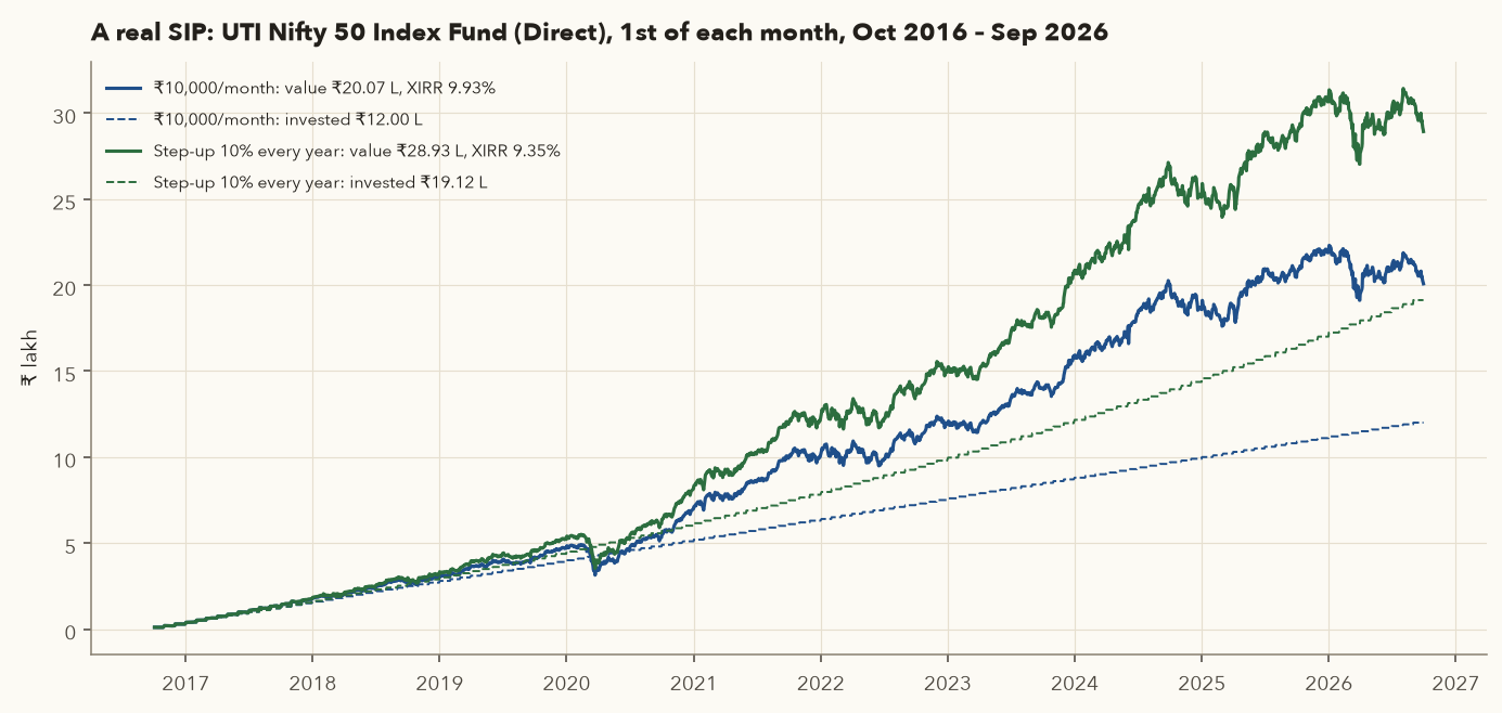
- First instalment, 3 Oct 2016 (1 Oct was a Saturday): NAV ₹55.9813. Units = 10,000 ÷ 55.9813 = 178.6311 (no stamp duty before July 2020).
- From 1 Jul 2020 each instalment loses 0.005% (₹0.50) to stamp duty: 9,999.50 ÷ NAV. Total stamp duty over the ten years: ₹37.50.
- After 120 instalments (last on 1 Sep 2026 at NAV ₹169.3801): 12,602.6214 units for ₹12,00,000.
- Average cost = 12,00,000 ÷ 12,602.6214 = ₹95.2183, against an average NAV paid of ₹110.2867. That is rupee-cost averaging at work.
- Value on 30 Sep 2026: 12,602.6214 × ₹159.2891 = ₹20,07,460.22, an absolute gain of 67.29%.
XIRR: the right return measure for a SIP
"67% in ten years" is misleading for a SIP: the first ₹10,000 was invested for ten years, the last for one month. Varsity's rule: for anything under a year use the absolute return; for a single lump sum over a year use CAGR (Chapter 1); for many cash flows at different dates use XIRR, the annual rate that makes the present value of all flows zero. (For a single lump sum, XIRR and CAGR are the same number.)
- \(i\)
- Which cash flow: each SIP instalment, any withdrawal, and finally today's value.
- \(C_i\)
- The cash flow in ₹. Money you put in is negative (it leaves your pocket); money you take out, or the current value at the end, is positive.
- \(d_i\)
- The date of cash flow \(i\). \(d_0\) is the date of the first one.
- \((d_i - d_0)/365\)
- How many years after the first cash flow this one happened (days ÷ 365).
- \(r\)
- The XIRR: the yearly return, as a fraction, that you are solving for.
- \(\sum_{i}\)
- "Add up over every cash flow."
- List every cash flow with its date and sign.
- Guess a rate \(r\). Divide each flow by \((1+r)\) raised to its age in years. This converts every flow back to its value on the first date.
- Add them up. If the total is above zero, the guess was too low; if below, too high. Adjust and repeat until the total is zero.
- That \(r\) is the XIRR: the single yearly rate that your money, taking into account when each rupee went in, has earned. Nobody does this by hand: use the spreadsheet
XIRR()function or the Python in part 17.
XIRR by hand, and why not to annualise short periods
- Cash flows: −10,000 on 3 Oct 2016 (NAV 55.9813, 178.6311 units), −10,000 on 1 Nov 2016 (55.3189, 180.7700 units), −10,000 on 1 Dec 2016 (52.5650, 190.2407 units).
- Value on 2 Jan 2017 at NAV 52.4637: 549.6418 units × 52.4637 = +₹28,836.24.
- Find \(r\) such that \(-10{,}000 - \frac{10{,}000}{(1+r)^{29/365}} - \frac{10{,}000}{(1+r)^{59/365}} + \frac{28{,}836.24}{(1+r)^{91/365}} = 0\). Trial and error (or a solver) gives r = −20.93%.
- The absolute return is only −3.88% (28,836.24 ÷ 30,000 − 1). Annualising three months of noise into "−21% a year" exaggerates it, which is exactly why short periods are quoted as absolute returns.
For the full ten-year SIP the XIRR is 9.93%. A lump sum invested on 3 Oct 2016 in the same fund would have compounded at 11.03% a year: higher, because all the money was in the market for the whole period.
The myth: "SIPs give better returns than lump sums"
A SIP smooths your entry price; it does not raise the expected return. Markets rise more often than they fall, so money invested earlier usually has more time to grow. The honest comparison is only for someone who already has a lump sum: invest it all now, or drip it in over 12 months through an STP (systematic transfer plan: park the money in a liquid fund and transfer a fixed amount into the equity fund each month)?
What the numbers say
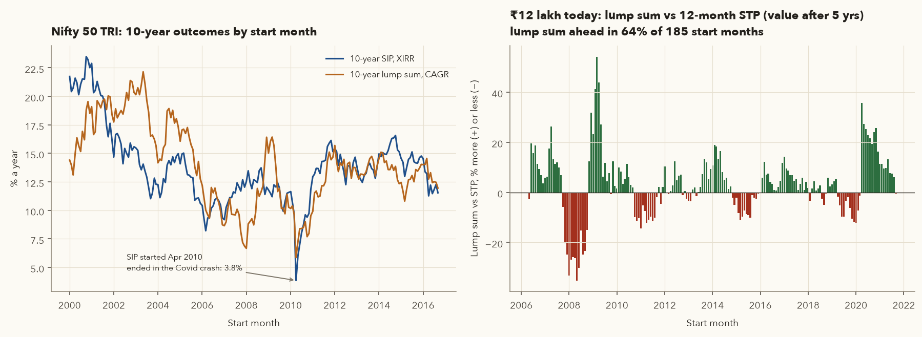
- Lump sum vs 12-month STP (₹12 lakh, liquid fund for the waiting money, value after 5 years, 185 start months from May 2006 to Sep 2021): the lump sum ended ahead in 63.8% of cases, by a median of 3.0%.
- But the losses were large when they came: starting in May 2008 the lump sum ended 35.17% behind; starting in Jan 2008 it was worth ₹12,29,296 after five years against ₹18,39,149 for the STP. The STP's value is insurance against regret, paid for with a lower average outcome.
- 10-year SIPs (201 start months, Jan 2000 – Sep 2016): median XIRR 13.52%, ranging from 3.85% (started Apr 2010, ended in the Apr 2020 Covid crash) to 23.49%. SIP XIRR beat the lump sum's CAGR in 51.7% of windows: a coin toss.
Take-away: invest monthly savings as they arrive (that is a SIP, and it is right). If you receive a large sum, investing it at once is better on average; spread it over 6–12 months only if a crash right after investing would make you abandon the plan.
Step-up SIP, STP and SWP
- Step-up (top-up) SIP: the instalment rises by a fixed percentage or amount each year, in line with income. The 10% step-up version of our SIP invested ₹19,12,490.95 (the last instalment ₹23,579.48) and was worth ₹28,92,664.62, XIRR 9.35%. It ends with more money because more was invested, and its XIRR is a little lower here only because more of the money went in during the expensive later years.
- STP: a transfer from one scheme to another in the same fund house each month, as above. Each transfer is a redemption from the source fund (a taxable event) and a purchase in the target.
- SWP (systematic withdrawal plan): the reverse of a SIP, redeeming a fixed amount each month, used in retirement. Each withdrawal redeems units, part capital and part gain, and only the gain is taxed. That is usually far more tax-efficient than an IDCW payout (part 13, Chapter 15). Withdraw more than the portfolio earns and you will run out; Chapter 16 covers safe withdrawal rates.
- Stopping the SIP after a fall. The months after a crash are when the SIP buys the most units. The 2020 dip in our SIP (value ₹5.33 lakh on ₹4.80 lakh invested in Sep 2020) was followed by its best year.
- Judging a 2-year-old SIP by its XIRR. Short-period XIRRs swing wildly.
- Running ten SIPs of ₹1,000 in ten similar funds. That is overlap, not diversification (part 14).
- Choosing a SIP date by superstition. Re-running our ten-year SIP on the 1st, 5th, 10th, 15th, 20th, 25th or 28th of each month gave XIRRs between 9.89% and 9.98%.
13. Growth vs IDCW, and a first look at fund tax
Each plan comes in two options:
- Growth: all income is reinvested and shows up as a rising NAV. You decide when to take money out (by redeeming units).
- IDCW (income distribution cum capital withdrawal, previously called the "dividend option"): the fund pays out cash from time to time and the NAV drops by the amount paid. SEBI renamed it in 2021 because the payout comes out of your own capital: it is not extra income.
For most investors growth is better: payouts are taxed at your slab rate as income from other sources, with 10% TDS (tax deducted at source) once a fund's payouts to you exceed ₹10,000 in a tax year (old s.194K; under the Income-tax Act, 2025 the TDS rules sit in s.393, as for share dividends in Chapter 13), and you lose control of timing. If you need regular cash, an SWP from the growth option usually costs far less tax, because only the gain portion of each withdrawal is taxed, and possibly at the lower capital-gains rates.
| Fund type (how the law classes it) | Short-term | Long-term |
|---|---|---|
| Equity-oriented (≥ 65% in Indian listed equity: Indian equity funds, Indian equity index funds and ETFs, ELSS, arbitrage funds, most balanced-advantage funds) | ≤ 12 months: 20% (new s.196, old s.111A) | > 12 months: 12.5% above ₹1.25 lakh a year (new s.198, old s.112A) |
| Specified mutual funds (more than 65% in debt and money-market instruments, e.g. liquid, gilt, corporate-bond funds; old s.50AA), bought from 1 Apr 2023 | Slab rate, however long you hold | |
| Other funds (gold and silver ETFs/FoFs, international funds, hybrids that are neither ≥ 65% equity nor > 65% debt; also debt-fund units bought before 1 Apr 2023) | Slab rate | 12.5%, no indexation, after 12 months (listed ETF units) or 24 months (unlisted FoF units) |
Plus 4% cess. These match the share rules in Chapter 13 and its other-assets table. Each SIP instalment is a separate purchase with its own holding period, and units are redeemed first-in-first-out. Chapter 15 covers lot-by-lot gains, grandfathering, LTCG and tax-loss harvesting with funds, and switching from regular to direct plans tax-efficiently. Ask a CA about your own situation.
14. How many funds? Portfolio overlap
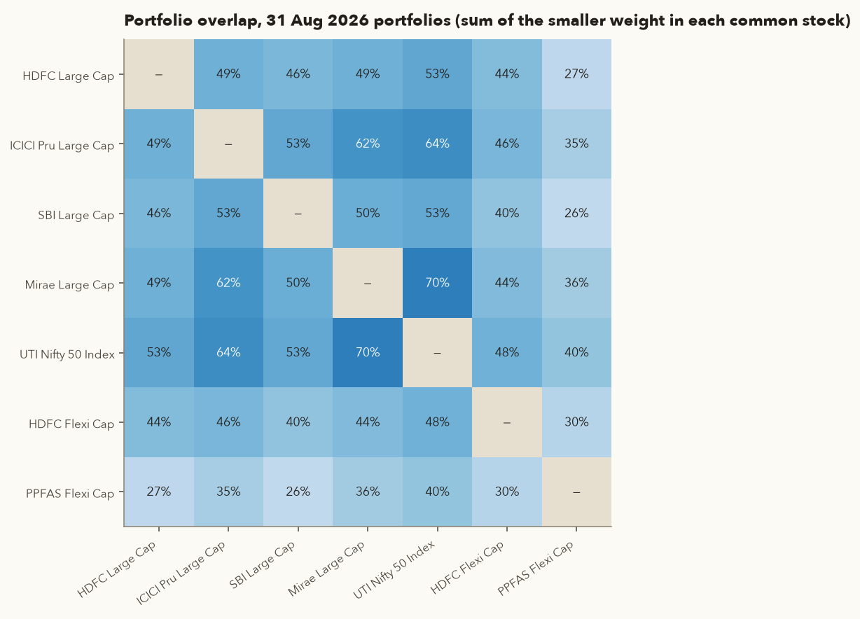
Diversification reduces risk only if the holdings are different (Chapter 11). Five large-cap funds are mostly the same 40 stocks, five times, with five fees. Portfolio overlap measures how much two funds hold in common.
- \(s\)
- One stock.
- \(A \cap B\)
- The stocks held by both fund A and fund B ("A intersect B").
- \(w_{A,s}\)
- The weight of stock \(s\) in fund A: its share of the fund's assets, in %, from the monthly portfolio disclosure. \(w_{B,s}\) is the same for fund B.
- \(\min\)
- The smaller of the two weights.
- \(\sum_{s \in A \cap B}\)
- "Add up over every stock the two funds share."
How it works: for each common stock, take the smaller of its two weights: that much of each fund is the same holding. Add these up. The result runs from 0% (nothing in common) to 100% (identical portfolios). The Mirae vs UTI example below gets 69.8%.
An active fund that is 70% index
- They share 32 stocks. The five biggest common holdings, as (Mirae %, UTI %) → min: ICICI Bank (8.97, 9.45) → 8.97; HDFC Bank (8.57, 9.85) → 8.57; Reliance (5.15, 7.83) → 5.15; Bharti Airtel (5.06, 5.00) → 5.00; Infosys (3.93, 3.61) → 3.61.
- Adding the smaller weight for all 32 common stocks gives 69.8%. Seven-tenths of the active fund is the index, yet its direct-plan TER (0.77%) is about three times the index fund's (0.25%). The active part, about 30% of the money, has to earn all the excess return.
A practical structure for most learners: three to five funds in total. For example, one broad equity index fund (or one flexi-cap fund), optionally one mid/small-cap or international fund as a small satellite, one debt fund (short duration, corporate bond or gilt, matched to your horizon) and a liquid fund for the emergency reserve. Varsity's portfolio chapter reaches the same conclusion: build by elimination, avoid two funds in the same sub-category, and review once a year rather than every month. How much goes into each, and how to rebalance, is Chapter 16.
15. Paperwork: KYC, CAS, MF Central, nomination, demat
- KYC (know your customer): one-time identity and address verification, recorded with a KYC Registration Agency (KRA) and shared across the industry. Since 2024 your status can be Validated (verified against official records such as Aadhaar or income-tax data; works everywhere), Registered (works with existing fund houses, may need re-verification for new ones) or On hold (fix it before investing). Link your PAN and Aadhaar, and keep mobile and email up to date.
- Folio: your account number with a fund house. One folio can hold all that AMC's schemes.
- CAS (Consolidated Account Statement): one statement of all your fund holdings across fund houses, sent by the depositories (if you have a demat account) or by CAMS/KFintech, every month in which you transact and every six months otherwise. The half-yearly CAS shows the commission paid on any regular-plan holdings, in rupees, and the scheme's TER. You can also request one any time from the RTAs' websites.
- MF Central: a joint platform of CAMS and KFintech where you can see all folios and make changes (bank account, nominee, contact details) and transact, across fund houses, in one place.
- Nomination: since SEBI's January 2025 circular (effective 1 Mar 2025), you may name up to 10 nominees per folio or demat account, with percentage shares. Without a nominee your family faces a long transmission process. (SEBI proposed further operational changes in March 2026; check the current form.)
- Demat or statement of account (SoA) mode? Funds can be held either way. SoA mode (the RTA's register) needs no demat account and lets you transact through MF Central or the AMC. Demat mode shows funds next to your shares, makes pledging easier and lets units be transferred, but ties transactions to your broker. ETFs are always held in demat.
16. Choosing a fund, step by step
Varsity's equity-fund analysis follows four checks: hygiene, rolling returns, risk-return and capture ratios. Here is a version for a beginner, in order.
- Start from the goal and horizon, not the fund. Money needed within 3 years does not belong in equity. Set the asset mix first (Chapter 16), then fill each slot.
- Pick the category for the slot. Core equity: a broad index fund or a flexi-cap fund. Debt matched to the horizon: liquid (under 6 months), money market or short duration (1–3 years), gilt or corporate bond (longer, if you accept rate swings).
- Passive first. If an index fund fits the slot, compare index funds on tracking difference over 1–3 years (part 10), then TER, then AUM. Choose an ETF instead only if you will check its iNAV and spread.
- For an active fund, run the hygiene check: direct plan; AUM neither tiny nor (for small-caps) enormous; the current manager's tenure; benchmark is a TRI; exit load; TER.
- Judge performance on rolling returns: 3- and 5-year rolling returns against the benchmark TRI and an index fund. How often did it beat it, by how much, and what was its worst period?
- Check the risk: standard deviation, beta and the worst drawdown against the benchmark. Excess return from much higher risk is not skill. Varsity also uses capture ratios: the share of the benchmark's up-months return the fund captured, and the share of its down-months losses. Upside above 100% and downside below 100% is the ideal.
- Check overlap with what you already hold (part 14). Below about 40% is genuinely different.
- For debt funds: YTM, Macaulay/modified duration against your horizon, credit quality (share of AAA and sovereign), concentration in any one issuer, and the PRC cell.
- Write down why you chose it and what would make you exit (a manager change, a style change, 3+ years of lagging its TRI on rolling returns). Review once a year, not every month.
17. In your framework, and try it yourself
The course framework has a framework.funds module for this part of the course. For this chapter: search_schemes(query) finds scheme codes; load_nav(scheme_code) downloads a NAV history from api.mfapi.in and caches it in data/mf/ (offline-first); cagr(series), rolling_returns(series, years) and xirr(cashflows) measure returns; sip_simulate(nav, amount, start, end=None, day=1, step_up_pct=0.0, stamp_duty=True) runs a SIP and returns its lots, value and XIRR; expense_drag(amount, years, gross_return, ter) and direct_vs_regular(amount, years, gross_return, ter_direct, ter_regular) do the cost arithmetic of parts 4–5 (they use the simpler approximation \(P(1+g-t)^n\), so their answers differ slightly from part 4's \(P[(1+g)(1-t)]^n\)); tracking_difference(fund, index) and tracking_error(fund, index) do part 10. All fund rates (stamp duty, STT, tax rates) live in framework/config.py. Run .venv/bin/python -m framework.funds --help for the command-line version. Chapters 15 and 16 use its tax, harvesting and rebalancing functions.
Run each snippet from the repository's root folder with .venv/bin/python snippet.py (setup in framework/README.md). Snippets 1 and 2 need only pandas and scipy and the CSVs saved in data/extra/; snippet 3 uses the framework.
1. A SIP and its XIRR, from a NAV file (reproduces part 12):
import pandas as pd
from scipy.optimize import brentq

nav = pd.read_csv("data/extra/ch14_mf_120716.csv", parse_dates=["date"]).set_index("date")["nav"]
nav = nav[~nav.index.duplicated()].sort_index()          # UTI Nifty 50 Index Fund - Direct - Growth

def xirr(flows):
    d0 = flows[0][0]
    f = lambda r: sum(a / (1 + r) ** ((d - d0).days / 365) for d, a in flows)
    return brentq(f, -0.99, 10)

lots = []
for d in pd.date_range("2016-10-01", "2026-09-01", freq="MS"):
    day = nav.index[nav.index.searchsorted(d)]           # next NAV date if the 1st is a holiday
    amt = 10_000 * (1 - 0.00005) if day >= pd.Timestamp("2020-07-01") else 10_000   # stamp duty
    lots.append((day, 10_000, amt / nav[day]))
units = sum(u for _, _, u in lots)
value = units * nav[:"2026-09-30"].iloc[-1]
flows = [(d, -a) for d, a, _ in lots] + [(pd.Timestamp("2026-09-30"), value)]
print(f"invested {sum(a for _, a, _ in lots):,.0f}  value {value:,.2f}  XIRR {xirr(flows):.2%}")
print(f"average cost {sum(a for _, a, _ in lots) / units:.4f}")
# -> invested 1,200,000  value 2,007,460.22  XIRR 9.93%  average cost 95.2183
2. Tracking difference, tracking error and an ETF's premium (reproduces part 10):
import numpy as np, pandas as pd

def nav(code):
    s = pd.read_csv(f"data/extra/ch14_mf_{code}.csv", parse_dates=["date"]).set_index("date")["nav"]
    return s[~s.index.duplicated()].sort_index()

tri = pd.read_csv("data/extra/ch14_nifty50_tri.csv", parse_dates=["Date"]).set_index("Date")["TRI"]
df = pd.concat([nav(140084), tri], axis=1, keys=["fund", "index"], join="inner")   # NIFTYBEES NAV vs TRI
d = df.loc["2021-09-30":"2026-09-30"]
yrs = 5
td = (d.fund.iloc[-1] / d.fund.iloc[0]) ** (1 / yrs) - (d["index"].iloc[-1] / d["index"].iloc[0]) ** (1 / yrs)
te = d.pct_change().dropna().pipe(lambda r: (r.fund - r["index"]).std() * np.sqrt(252))
print(f"NIFTYBEES 5-yr tracking difference {td:.3%}, tracking error {te:.3%}")   # -0.044%, 0.031%

price = pd.read_csv("data/extra/ch14_MON100_yf.csv", index_col=0, parse_dates=True)["Close"]
m = pd.concat([price, nav(114984)], axis=1, keys=["p", "n"], join="inner").dropna().loc["2022":]
m["premium"] = m.p / m.n - 1
print(m.premium.describe().round(4))
print("MON100 premium on 30 Sep 2026:", round(m.premium.iloc[-1] * 100, 2), "%")    # 12.73 %
3. The same with the framework (downloads NAVs into data/mf/ the first time):
import sys; sys.path.insert(0, ".")      # run from the repository root, so framework/ is importable
from framework.funds import search_schemes, load_nav, sip_simulate, rolling_returns, direct_vs_regular

print(search_schemes("hdfc flexi cap direct growth").head())
r = sip_simulate(load_nav(120716), 10_000, "2016-10-01", end="2026-09-30")
print(r["invested"], r["value"], round(r["xirr"] * 100, 2))
# -> 1200000.0 2007460.22 9.93  (stamp duty only from 1 Jul 2020, matching part 5)
roll = rolling_returns(load_nav(118955), 5)            # HDFC Flexi Cap Direct, rolling 5-yr CAGR
print(roll.describe())
d = direct_vs_regular(10_00_000, 20, 0.12, 0.0077, 0.0155)  # Rs 10 lakh, 20 yrs, 12% gross
print(d["direct"], d["regular"], d["difference"])     # -> 8403084.76 7299857.87 1103226.9
Exercise: pick one fund you own (or want to own). Find its direct and regular codes with search_schemes, compute the 5-year CAGR gap between the plans, its 3-year rolling returns against the right TRI, and its tracking difference if it is an index fund. Would you still choose it?
The full chapter calculation, with every number quoted above, is course/scripts/ch14_figures.py; its output is saved to data/extra/ch14_numbers.json.
18. Practical checklist
- KYC status "Validated"; PAN–Aadhaar linked; mobile, email and bank account current; nominees added on every folio and demat account.
- Every fund you hold is a direct plan, unless you knowingly pay a distributor for advice you use.
- Every equity fund is judged against its TRI, on 3- and 5-year rolling returns, not last year's return.
- For each index fund or ETF: tracking difference over 1 and 3 years, TER, and (ETF) average spread and volume checked.
- Before any ETF order: compare the price with the iNAV; use a limit order; avoid the first and last 15 minutes of the session.
- Debt funds chosen by horizon: Macaulay duration no longer than the time until you need the money; credit quality mostly AAA/sovereign; no single issuer above about 10%.
- Emergency money in a liquid or overnight fund (or a bank deposit), not in a gilt, credit-risk or equity fund.
- No more than 3–5 funds; overlap between equity funds checked once a year.
- Growth option chosen; if you need income, an SWP rather than IDCW.
- Exit loads and 12/24-month tax dates checked before any redemption or switch (Chapter 15).
- SIPs keep running through falls; a large windfall is invested at once or through a short STP, by a written rule.
- The half-yearly CAS reviewed: holdings, commissions, TERs, nominees.
- After each SEBI change (TER, categories) and each Budget, re-check your funds' notices and
framework/config.py.
19. Key takeaways
- A mutual fund is a trust: the AMC manages, a custodian holds, trustees supervise, an RTA (CAMS/KFintech) keeps the books, under SEBI's rules.
- NAV = net assets ÷ units, computed daily after expenses. The NAV level means nothing; a ₹10 NFO is not cheaper than a ₹170 fund.
- Costs compound: on ₹10 lakh over 25 years, a 1.6% TER instead of 0.2% cost ₹38.45 lakh. From 1 Apr 2026, SEBI caps the AMC's base expense ratio (BER) lower and shows levies separately.
- Regular plans cost about 0.8–0.9% a year more on real NAVs: on a ₹10,000 ten-year SIP, ₹1.14–1.41 lakh.
- Categories define what a fund must hold. New in 2026: life cycle (target-date) funds; SIFs from 2025 for ₹10 lakh+ investors.
- Debt funds move with yields: price change ≈ −modified duration × change in yield. A long gilt fund lost 1.12% in a quarter when yields rose 0.43 points. Credit and liquidity risk can freeze money (Franklin, 2020).
- Active vs passive: over 10 years only 11 of 27 large-cap funds beat the Nifty 100 TRI and 6 vanished; SPIVA's 10-year underperformance rate is 76.3%. Judge on rolling returns and beware survivorship bias.
- Tracking difference is what an index product costs you (NIFTYBEES −0.04% a year, a regular index fund −0.36%); tracking error is how unevenly it follows.
- ETFs can trade far from NAV when creation is blocked: MON100 at a 22% premium in Dec 2024 and 12.7% on 30 Sep 2026. Check iNAV, use limit orders.
- A SIP is a habit, not a return booster: a lump sum beat a 12-month STP in 64% of cases. Measure SIPs with XIRR (our 10-year Nifty SIP: 9.93%).
- Prefer the growth option; hold 3–5 funds with low overlap; keep KYC, nominees and the CAS in order.
20. Quiz and exercises
Q1. A scheme holds securities worth ₹480 crore, cash of ₹12 crore and has liabilities of ₹2 crore. There are 20 crore units. What is the NAV, and how many units does ₹50,000 buy after stamp duty?
NAV = (480 + 12 − 2) crore ÷ 20 crore = 490 ÷ 20 = ₹24.50. Stamp duty = 0.005% × 50,000 = ₹2.50, so ₹49,997.50 is invested: 49,997.50 ÷ 24.50 = 2,040.714 units.
Q2. You place a ₹1 lakh purchase in an equity fund at 2:50 pm, but your bank transfer reaches the fund at 3:20 pm. Which NAV do you get? What if it were a liquid fund order placed at 1:00 pm with money arriving at 1:10 pm?
For non-liquid funds, the NAV applies to the day the money is realised in the scheme before the 3:00 pm cut-off. The money arrived after 3:00 pm, so you get the next business day's NAV. For the liquid fund, both the order and the money arrived before 1:30 pm, so you get the NAV of the day before the money arrived (liquid and overnight funds accrue interest daily, so you earn from that day).
Q3. ₹5 lakh grows at 12% gross for 20 years. What is the final value with a TER of 0.5% and of 1.5%, and the difference?
0.5%: 5,00,000 × (1.12 × 0.995)20 = 5,00,000 × 1.114420 ≈ 5,00,000 × 8.73 ≈ ₹43.6 lakh. 1.5%: 5,00,000 × (1.12 × 0.985)20 = 5,00,000 × 1.103220 ≈ 5,00,000 × 7.12 ≈ ₹35.6 lakh. Difference ≈ ₹8 lakh, more than the ₹5 lakh invested. (Gross, with no costs: 5,00,000 × 1.1220 ≈ ₹48.2 lakh.)
Q4. HDFC Flexi Cap's direct plan returned 15.52% a year over 10 years and its regular plan 14.72%. On a ₹10 lakh lump sum, roughly how much more would the direct plan be worth after 10 years?
Direct: 10,00,000 × 1.155210 ≈ 10,00,000 × 4.23 ≈ ₹42.3 lakh. Regular: 10,00,000 × 1.147210 ≈ 10,00,000 × 3.95 ≈ ₹39.5 lakh. About ₹2.8 lakh more, from a 0.80% yearly difference. (The actual NAVs show the direct plan's NAV ran about 9.9% ahead of the regular plan's since June 2013.)
Q5. A debt fund has a modified duration of 4 years and a YTM of 7.2%. Yields jump by 0.75 percentage points in a week. Roughly how much does the NAV fall? Over the next year, if yields stay there, what return would you expect?
Price effect ≈ −4 × 0.75% = −3.0% in the week (ignoring the week's tiny carry). After that, the portfolio yields about 7.2 + 0.75 = 7.95%, so over the next year you would expect roughly 7.95% minus the TER. Holding for about the duration lets the higher yield make up the loss; selling right after the jump locks it in.
Q6. A friend says: "My large-cap fund beat the Nifty 50 by 2% a year over the last 3 years, so active funds clearly beat index funds." What three things would you check?
(1) The right benchmark: large-cap funds are judged against the Nifty 100 TRI (or BSE 100 TRI), not the Nifty 50 price index, which leaves out dividends (worth roughly 1–1.5% a year). Over 3 years to Sep 2026 the Nifty 100 TRI (7.81%) beat the Nifty 50 TRI (6.06%) by about 1.75% a year, so most of the "2%" came from the benchmark choice. (2) Rolling returns over longer periods: over 10 years only 11 of 27 large-cap funds beat their benchmark. (3) Survivorship: funds that did badly were merged away and are missing from the list your friend compares against.
Q7. An ETF's NAV is ₹250.00 and it trades at ₹262.50. What is the premium? If you buy and the premium disappears while the NAV rises 10%, what is your return?
Premium = (262.50 − 250.00) ÷ 250.00 = 5.0%. New NAV = 275.00; with no premium the price ≈ ₹275.00. Your return = 275.00 ÷ 262.50 − 1 = 4.76%, less than half of the 10% the holdings earned. Check the iNAV before buying and avoid ETFs trading at a persistent premium.
Q8. Index fund A has a TER of 0.20% and a 3-year tracking difference of −0.25% a year. Index fund B has a TER of 0.15% and a tracking difference of −0.40%. Which would you choose, and why might B lag more than its TER?
Choose A: tracking difference is the return you actually lost, and A lost 0.15% a year less. B's extra lag beyond its TER can come from cash drag (holding cash for inflows and outflows), trading costs when the index changes, poor handling of corporate actions, or a TER that was cut only recently (the past TD reflects the old, higher TER). Re-check yearly.
Q9. You invested ₹10,000 on 1 Jan and ₹10,000 on 1 Jul, and the holding is worth ₹21,500 on 31 Dec. Your app shows "7.5% returns". What is the absolute return, and is the XIRR higher or lower than 7.5%?
Absolute return = 21,500 ÷ 20,000 − 1 = 7.5%; that is what the app shows. The XIRR is higher: the second ₹10,000 was invested for only half a year, so the average money invested was about ₹15,000 for a year. Solving \(-10{,}000 - 10{,}000/(1+r)^{181/365} + 21{,}500/(1+r)^{364/365} = 0\) gives r ≈ 10%. For periods under a year, report the absolute return; for SIPs over a year, use XIRR.
Q10. You receive a ₹15 lakh bonus and plan to invest it in an equity index fund for 10 years. Your colleague says "always SIP it over 12 months". What does the data in part 12 suggest?
Over 185 five-year windows since 2006, investing a lump sum at once beat a 12-month STP in 63.8% of cases (median +3.0%). But in bad starts (2008) the lump sum ended up to 35% behind. So: investing at once is better on average; an STP over 6–12 months is reasonable if a crash right after investing would make you sell. Whichever you choose, decide in advance and write it down. Keep the waiting money in a liquid fund, not a savings account.
Q11. Fund X holds HDFC Bank 9%, ICICI Bank 8%, Reliance 6%, Infosys 5%. Fund Y holds HDFC Bank 6%, ICICI Bank 10%, TCS 7%, Infosys 3%. Considering only these stocks, what is their overlap?
Common stocks: HDFC Bank min(9, 6) = 6; ICICI Bank min(8, 10) = 8; Infosys min(5, 3) = 3. Reliance and TCS are not common. Overlap = 6 + 8 + 3 = 17% of the portfolio from these names. In real large-cap funds the total is usually 45–70% (part 14).
Q12. A retired relative wants ₹25,000 a month from a ₹40 lakh hybrid fund. Should they choose the monthly IDCW option or a growth option with an SWP? Why?
Usually growth + SWP. IDCW payouts are not guaranteed (the fund decides the amount), are taxed in full at the slab rate, and attract 10% TDS once a fund house pays you more than ₹10,000 in a year. With an SWP, each ₹25,000 redemption is mostly the original capital in the early years; only the gain part is taxed, at capital-gains rates that depend on the fund's class and holding period. The amount is predictable. Check that ₹3 lakh a year (7.5% of ₹40 lakh) is sustainable (Chapter 16) and ask a CA about the tax.
Q13. Exercise: download your CAS. For each holding, note the plan (direct or regular), category, TER, and benchmark. Which changes would this chapter suggest?
Open-ended. Check: (1) any regular plans, and the rupee commission the CAS shows for each; (2) more than one fund in the same sub-category (overlap); (3) sectoral or thematic funds above a small satellite share; (4) debt funds whose duration is longer than your horizon, or credit-risk funds; (5) IDCW options you do not need; (6) missing nominees. Before switching anything, check exit loads and the tax on the switch (Chapter 15).
21. Sources
Zerodha Varsity, Module 11, Personal Finance – Mutual Funds (concepts; explained here in our own words and updated to 2026 rules): 6. Mutual Funds Introduction · 7. Concept of Fund NAV · 8. The Mutual Fund Fact Sheet · 9. Equity Scheme (Part 1) · 10. Equity Scheme (Part 2) · 11–14. Debt Funds (Parts 1–4): 2, 3, 4 · 17. Arbitrage Funds · 18. Measuring Mutual Fund Returns · 19. Rolling Returns · 20. Expense Ratio, Direct and Regular Plans · 21. Mutual Fund Benchmarking · 22. Risk Metrics · 23. Sortino and Capture Ratios · 24. How to Analyse an Equity Fund · 25. How to Analyse a Debt Fund · 26. The Mutual Fund Portfolio · 27. Smart-Beta Funds · 28. Index Funds · 29. Exchange Traded Funds · 33. Know Your Fund.
Regulation and rules (checked 2 Oct 2026): Kotak MF: SEBI (Mutual Funds) Regulations 2026 BER slab limits · INDmoney: SEBI MF Regulations 2026 (board approval 17 Dec 2025; index/ETF 1.00%→0.90%; exit-load 0.05% removed; brokerage caps) · Cafemutual: the new expense framework from 1 Apr 2026 · Upstox: fund houses revise expense ratios as the 2026 rules start · Taxmann: SEBI circular of 26 Feb 2026 on categorisation · Angel One: life cycle funds, 50% overlap caps, residual in gold/silver/InvITs · Finnovate: life cycle fund glide paths and exit loads · 5paisa: SEBI allows retirement and children's funds to continue (20 Mar 2026) · Upstox: REITs as equity for mutual funds from 1 Jan 2026 · Value Research: Specialised Investment Funds (₹10 lakh minimum) · PwC: SEBI's 2017 categorisation circular explained · Bajaj Finserv AMC: cut-off times and NAV applicability · A scheme information document on AMFI's portal (redemption within 3 working days; AMFI letter of 16 Jan 2023) · SEBI-filed ETF document: direct dealing with the AMC above ₹25 crore; market makers · Moneylife: up to 10 nominees (SEBI circular, 10 Jan 2025) · Vested: SEBI limits on overseas investment by mutual funds · ClearTax: Sovereign Gold Bonds, no new issues; Budget 2026 change to the redemption exemption · Taxguru: TDS threshold on fund income raised to ₹10,000 from 1 Apr 2025 · Income Tax Department: section 50AA (specified mutual funds) · TaxTMI: amended definition of specified mutual fund (more than 65% debt).
Evidence and episodes: S&P Dow Jones Indices: SPIVA India Scorecard, Year-End 2025 · Angel One: SPIVA India Mid-Year 2025 summary · Franklin Templeton India: winding up of six schemes (₹27,548.21 crore, 109.25% of AUM distributed) · Business Standard: silver ETFs at steep premiums (Oct 2025) · Moneylife: fund houses pause silver FoF subscriptions.
Data: mutual-fund NAVs from AMFI via api.mfapi.in (saved as data/extra/ch14_mf_<code>.csv; every large-cap direct plan, live and closed, in data/extra/ch14_largecap_direct_navs.csv); Nifty 50 and Nifty 100 Total Return Index from niftyindices.com (data/extra/ch14_nifty50_tri.csv, ch14_nifty100_tri.csv); ETF prices from NSE via Yahoo Finance (data/extra/ch14_*_yf.csv, NIFTYBEES/GOLDBEES from data/extra/); portfolios as of 31 Aug 2026 and TER/AUM figures from Groww's public scheme pages, 1 Oct 2026 (data/extra/ch14_holdings_groww.csv, ch14_fund_facts_groww.csv); 10-year G-sec yields from countryeconomy.com (data/extra/ch08_india_10y_gsec_monthend_countryeconomy.csv). All calculations and figures: course/scripts/ch14_figures.py (numbers in data/extra/ch14_numbers.json). Examples are historical and educational, not recommendations.