
Build Your Own Framework
1. What you'll learn and why it matters
The previous sixteen chapters gave you separate skills: reading charts, measuring trends, reading a balance sheet, valuing a business, pricing a future, sizing a position, paying the right tax, choosing a fund and setting an allocation. Skills on their own do not make anyone a consistent trader or investor. What does is a process: written rules for what you buy, how much, when you get out and how you check yourself, followed the same way on good days and bad days.
This capstone turns the course into that process. It uses the actual Python code in the course repository's framework/ folder (the toolkit built alongside this course; its README.md explains how to install it) and the actual market data up to 30 September 2026. Every output shown below is real: the scanner's output for 30 Sep 2026, the scorecards for TCS, Pidilite, HDFC Bank and ITC, the backtests, and a learner's own strategy idea that we design, test and, in the end, reject.
By the end you will be able to:
- Split your money into three buckets (long-term core, swing satellite, futures) with separate rules, and know when you are allowed to move up from paper trading to small size, normal size and futures.
- Run the long-term pipeline: universe, screen, checklist, valuation and buy zones, sizing, quarterly review and sell rules, using
python -m framework.invest. - Run the swing pipeline every evening: market regime, scanner, setup check, position size, GTT orders, management, journal and weekly review, using
python -m framework.scanandpython -m framework.journal. - Decide when futures make sense, size them by lot and stop, keep a margin buffer and hedge a portfolio with Nifty futures.
- Read backtest results honestly and test your own strategy idea with the template, a causality test and robustness checks.
- Write your own trading plan, follow daily/weekly/monthly/quarterly routines and work through a 12-week roadmap that starts with paper trading.
Retail traders rarely fail for lack of indicators. They fail because they size too big, change rules after every loss, skip the journal and trade products (like F&O) before they have shown an edge anywhere. SEBI's July 2025 study found that 91% of individual equity F&O traders made a net loss in FY2024-25, with aggregate net losses of about Rs 1.06 lakh crore. A framework is how you avoid becoming part of that number: it makes the risky decisions in advance, while you are calm.
Every stock named here is a historical, educational example computed from data to 30 Sep 2026. Nothing in this chapter is a recommendation to buy or sell anything. Allocation percentages are teaching examples; your own numbers depend on your income, obligations, tax situation and temperament.
2. What a trading system is, and what your framework contains
Varsity's Module 10 opens with a useful distinction. Many people trade on a hunch, a friend's tip, a TV guest or a broker's call. Even a sensible-sounding "systematic deduction" ("PSU banks jumped, so Bank Nifty overreacted") is still ad hoc if you cannot write it down as a repeatable procedure. A trading system is an approach you can define as a process: it takes inputs (prices, volumes, financial data), applies fixed logic, produces an output (a list of trades, a size, a stop), and you decide, or the system decides, whether to act. Varsity is also clear about two things. A system is not a money machine, because you design it, you feed it and you choose to follow it. And no system is complete until it has been backtested.
The framework/ package is exactly such a system, split into small modules that each correspond to a part of this course:
| Course chapter | What you learned | Framework code | How you use it |
|---|---|---|---|
| 1 Market foundations | NSE, settlement, corporate actions | config.py, data.load_ohlc (back-adjusts missed corporate actions) | Clean data in, everything else depends on it |
| 2-4 Charts, S/R, indicators | Candles, trends, RSI, ATR, MAs | indicators.py, patterns.py | Building blocks for every rule |
| 5 Swing playbook | Regime, RS, setups, GTT | strategies.py, scan.py | python -m framework.scan every evening |
| 6-8 Fundamentals, ratios, valuation | Statements, DuPont, Piotroski, DCF | fundamentals.py, invest.py | python -m framework.invest SYMBOL |
| 9-10 Futures, options | Carry, OI, margins, hedging | futures.py, run_futures_backtest | Hedge calculator, OI context, MTM ledger |
| 11 Risk & psychology | Position size, R, expectancy, ruin | risk.py, journal.py | Every order's quantity; your honest scorecard |
| 12 Systems & backtesting | No look-ahead, costs, robustness | backtest.py, backtest_cli.py | python -m framework.backtest_cli NAME |
| 13 Costs & tax | STT, stamp duty, STCG/LTCG | costs.py (rates only in config.py) | Every backtest and journal entry is net of costs |
| 14-16 Funds, fund tax, allocation | NAV, TER, SIP and XIRR, fund tax classes, harvesting, rebalancing | funds.py | python -m framework.funds sip, tax, harvest, rebalance |
Data flows in one direction, which is what keeps the system honest (no module can peek at the future):
 data.load_ohlc ──> indicators / patterns ──> strategies (entry, exit, stop, trail, score per bar)
                                                      │
                     risk.position_size  <────────────┤
                     costs.*_charges     <── backtest.run_backtest ──> trades, equity, metrics ──> reports/
                                                      │
                                     scan.py (today's bar only) ──> you ──> journal.py
 fundamentals.fetch_fundamentals ──> ratios / dupont / piotroski / scorecard / dcf ──> invest.py
 data.load_futures ──> futures.oi_buildup_table / rollover_pct / fair_value / beta_hedge
 funds.load_nav ──> sip_simulate / fund_capital_gains / harvest_plan / rebalance_backtest
Before relying on it, check that the code does what it claims. The framework ships with a test suite, including a test that fails if any strategy uses future data:
$ .venv/bin/python -m pytest framework/tests -q
129 passed in 1.15s
Every command in this chapter runs from the repository's root folder. .venv/bin/python is the project's own Python (a virtual environment created during setup); where a command just says python, use that same interpreter. Each command also accepts --help.
For every position you ever hold, your framework should already have answered: (1) why this instrument, now (the entry rule), (2) how much (the sizing rule) and (3) what makes me get out, both when wrong (stop) and when right (exit or trail). If any of the three is "I'll see", it is not a framework yet.
3. The three-bucket structure and capital allocation
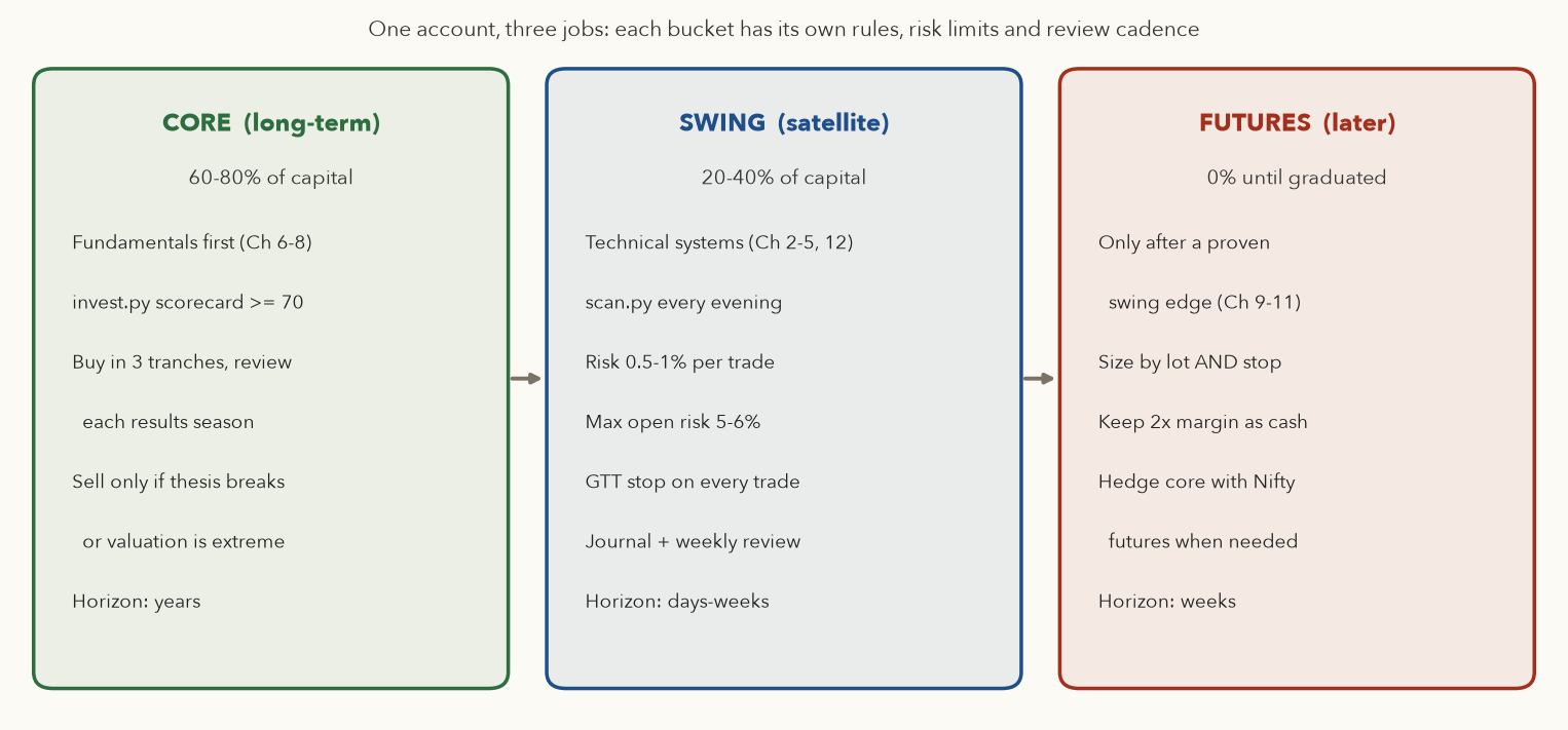
You told this course you want swing trades, long-term positions and, slowly, futures. These are three different jobs with different edges, holding periods and risks, so they get three separate buckets with their own rules.
Why separate buckets? The logic
- Different sources of return. The core earns from business growth over years, either through stocks you research (Chapters 6-8) or through index funds that own the whole market (Chapters 14-16). The swing bucket tries to earn from price trends lasting days to weeks (Chapters 2-5). Futures add leverage and the ability to hedge or go short (Chapter 9). Mixing them causes classic mistakes, such as turning a failed swing trade into a "long-term investment" to avoid booking a loss.
- Different risk units. In the core, risk is controlled by diversification and position weight (no single stock above about 10%). In the swing bucket it is controlled per trade by a stop and the 1% rule. In futures it is controlled by stop, lot size and a margin buffer, because leverage turns a normal move into a large rupee loss.
- Different review cadence. The core is reviewed after each quarterly result. Swing trades are reviewed daily and weekly. Mixing cadences leads to over-trading the core and under-supervising trades.
An educational allocation example
Before any bucket: keep an emergency fund (commonly six months of expenses) and adequate insurance outside the market. Only money you will not need for at least five years belongs in the core, and only money you can afford to lose part of belongs in the swing bucket. Suppose, after that, you have Rs 10 lakh to invest:
| Bucket | Stage 0-1 (first 6-12 months) | Stage 2 (proven swing edge) | Risk unit |
|---|---|---|---|
| Core (long-term) | Rs 8.0 lakh (80%), staggered in over 6-12 months | Rs 7.0 lakh (70%) | Max 10% of core per stock, 25-30% per sector |
| Swing satellite | Rs 2.0 lakh (20%), real money only from Stage 1 | Rs 3.0 lakh (30%) | 0.25% (Stage 1) to 1% (Stage 2) of the swing bucket per trade |
| Futures | 0 | 0 until Stage 3 | Lot-and-stop sizing; at least 2x margin in cash |
The swing bucket's risk per trade is a percent of that bucket's capital, not your total wealth. This is Varsity Module 9's point about defining equity capital before you size anything. Varsity describes three ways to measure it: core equity (starting capital minus money committed to open trades), total equity (cash plus open positions marked to market) and reduced total equity (core equity plus only the profit already locked in by trailing stops, as defined in Chapter 5). The framework's backtester uses total equity marked to market at the previous close. Whichever you choose, write it in your plan and use it every time.
- \(C\)
- The capital of the bucket you are trading from (the swing bucket, not your total wealth), in Rs.
- \(r\)
- Risk per trade as a percent of \(C\): 0.25 at Stage 1, up to 1 at Stage 2. Dividing by 100 turns it into a fraction.
- \(m\)
- The regime multiplier from the scanner: 1 (Risk-on), 0.5 (Neutral) or 0.25 (Risk-off).
- \(E\)
- The entry price per share, in Rs. (In section 4, \(E\) means expectancy: a different quantity.)
- \(S\)
- The stop-loss price per share, in Rs. For a long trade \(E - S\) is the rupees you lose per share if the stop is hit.
- \(\lfloor\ \ \rfloor\)
- "Floor": round down to a whole number of shares (or whole lots for futures).
- \(p_{\max}\)
- The largest position allowed, as a percent of \(C\). The framework's backtester and scanner use 20.
- qty
- The number of shares to buy.
- Rupees you are willing to lose on this trade: \(C \times r/100 \times m\).
- Divide by the loss per share \((E - S)\) and round down. If the stop is hit, you lose about the planned amount.
- Check the cap: if qty × entry is more than \(p_{\max}\)% of the bucket (a very tight stop gives a huge quantity), cut qty to fit. If the answer is 0, the trade is too big for the account.
Example (illustrative entry and stop): Rs 2 lakh bucket, Stage 2 risk 1%, Risk-off regime (\(m\) = 0.25, as on 30 Sep 2026), entry Rs 1,000, stop Rs 950. Risk = 2,00,000 × 1/100 × 0.25 = Rs 500. Qty = 500 ÷ 50 = 10 shares, a Rs 10,000 position, well under the 20% cap of Rs 40,000.
How much is "1%"?
- Stage 1 risk: \(2{,}00{,}000 \times 0.25\% = \) Rs 500 per trade. At Stage 2 with 1%: Rs 2,000.
- Maximum open risk at Stage 2, if you cap it at 6%: \(2{,}00{,}000 \times 6\% = \) Rs 12,000, which is about six full-risk trades at once.
- Worst realistic streak: the best system in the framework's backtest (
donchian_trend) had a longest run of 18 consecutive losing trades in nine years. At 1% each, that is roughly a 16.5% drawdown of the bucket (\(0.99^{18} = 0.835\)). At 5% per trade it would be about 60% (\(0.95^{18} = 0.397\)). That is the whole argument for small risk per trade.
Varsity Module 9 shows why protecting capital comes first: after a loss of \(d\), you need a gain of \(\frac{1}{1-d} - 1\) to get back. Nifty's fall from its 2 Jan 2026 high of 26,328.55 to 22,620.45 on 30 Sep 2026 is -14.1%, which needs +16.4% to recover. The donchian_trend backtest's -27.0% drawdown needs +37.0%. A 50% loss needs +100%.
4. Graduating between stages: how many trades is enough?
The biggest beginner question is "when do I start with real money, and when do I increase size?" The honest answer is statistical: only when your sample of trades is large enough to show that your edge is probably real. Here is the ladder used in this course.
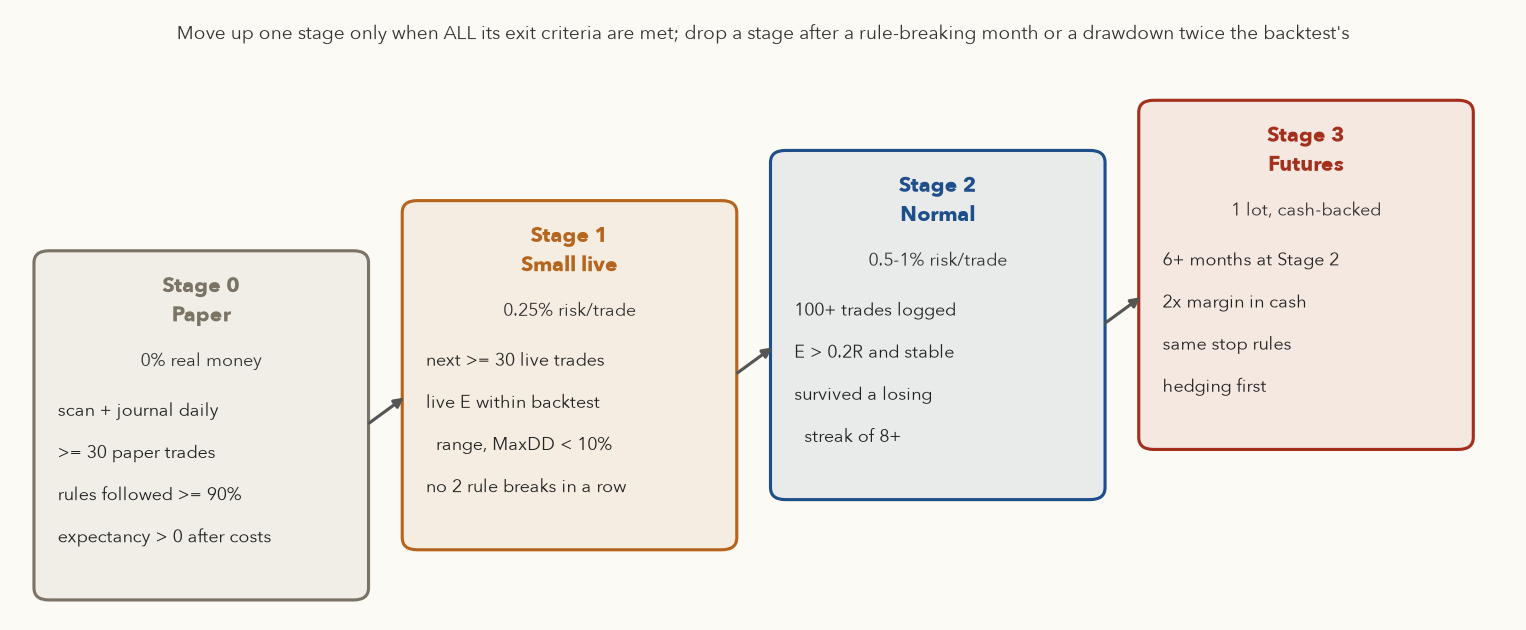
The logic: expectancy is measured with error
First, the unit. An R-multiple is a trade's profit or loss divided by the rupees you planned to risk on it (quantity x (entry - stop)). If you risked Rs 1,000 and lost Rs 1,000, that trade was -1R; if you made Rs 2,500, it was +2.5R. Expectancy (Chapter 11) is the average R-multiple per trade. With few trades it is very noisy, because swing results are lopsided: many small losses and a few large wins. The uncertainty of your measured expectancy is its standard error:
- \(E\)
- Your expectancy: the average R-multiple of all your trades so far, in R.
- \(s_R\)
- The standard deviation of your R-multiples, in R: how widely individual trade results spread around the average.
- \(n\)
- The number of trades in your sample.
- \(\sqrt{n}\)
- The square root of \(n\). Four times as many trades halves the error.
- \(SE\)
- The standard error of the expectancy, in R: roughly how far your measured average could be from the true one, just by luck.
- \(1.645\)
- The z-value for 95% one-sided confidence (equivalently, a two-sided 90% interval) under a normal curve.
- \((\dots)^2\)
- "Squared": the bracket multiplied by itself.
- \(n_{\min}\)
- The number of trades needed before \(E > 0\) is significant at about 95% confidence (one-sided).
- Compute \(E\) and \(s_R\) from your trade list (a spreadsheet's
AVERAGEandSTDEVon the R column). - Divide \(s_R\) by \(\sqrt{n}\) to get \(SE\). Your true edge probably lies within \(E \pm 1.645 \times SE\).
- If that range still includes zero, you cannot yet tell your edge from luck. \(n_{\min}\) is the sample size at which the lower end just reaches zero: it is the \(n\) that makes \(1.645 \times SE = E\). Lopsided results (big \(s_R\)) or a thin edge (small \(E\)) need many more trades.
How sure can we be about a +0.50R edge?
- Trades: \(n = 363\). Expectancy \(E = 0.498\)R. Standard deviation \(s_R = 3.595\)R (one trade made +29.26R; the median trade was -1.04R; only 31.1% of trades won).
- \(SE = 3.595 / \sqrt{363} = 0.189\)R, so a 90% interval is \(0.498 \pm 1.645 \times 0.189\) = 0.19R to 0.81R. Positive, but wide.
- Trades needed: \((1.645 \times 3.595 / 0.498)^2 = 141.0\), round up to 142 trades. A trend system with a few big winners needs well over a hundred trades before you can trust it.
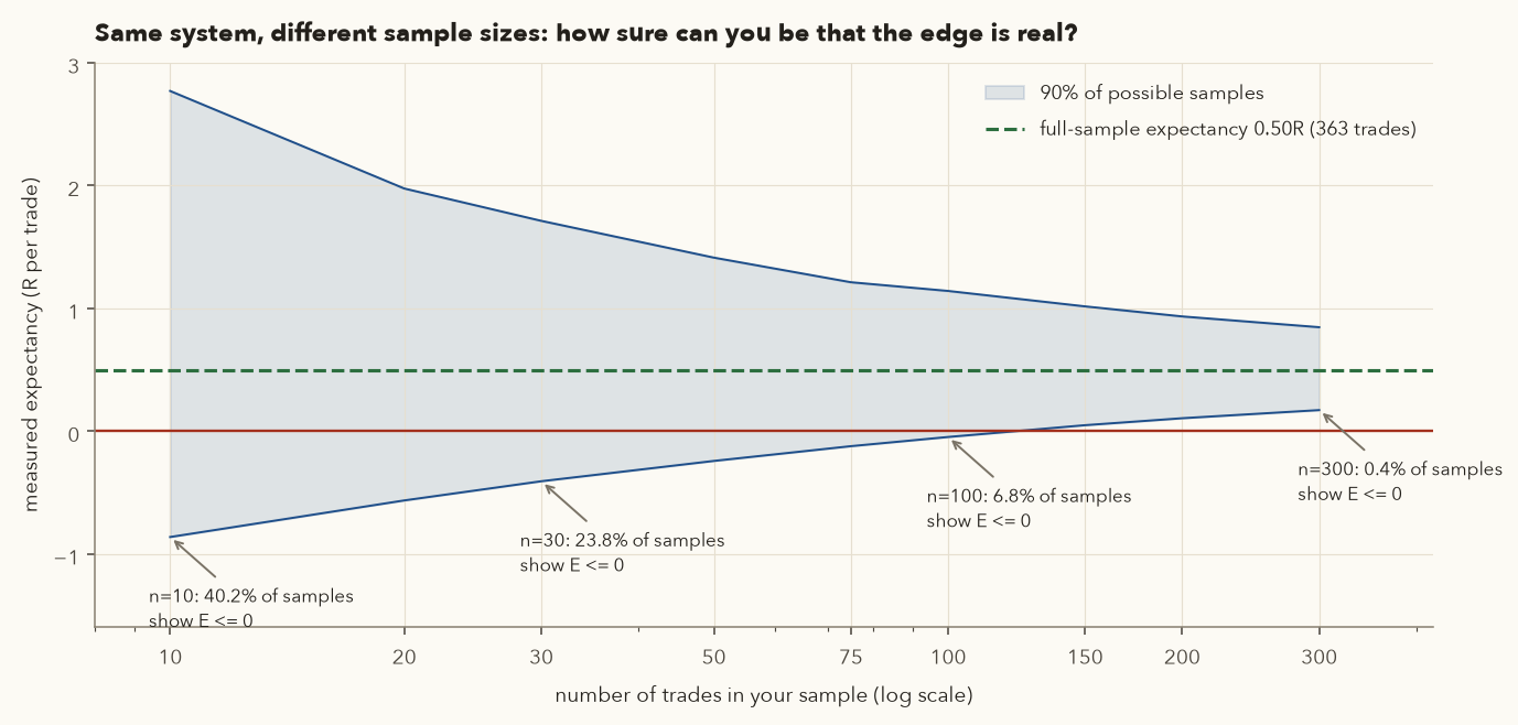
donchian_trend trades: with 30 trades, almost one sample in four shows a losing system even though the full-sample edge is +0.50R. Source: framework/reports/donchian_trend_trades.csv.This is why the ladder asks for at least 30 paper trades before small live money (to check you can follow the rules and that nothing is broken), and 100+ trades before full size. Thirty trades cannot prove an edge. They can reveal execution problems and rule-breaking.
Demotion: when the edge seems to have gone
Graduation runs both ways. Compare your live results with the backtest's distribution, and step down if live results fall outside it.
A good system going through a very bad patch
- "Backtest" sample (entries before 2025): 275 trades, expectancy +0.75R.
- "Live" sample (entries from 2025 to Sep 2026): 88 trades, expectancy -0.29R, win rate 22.7%.
- Resample 88 trades from the older 275 many times (50,000 draws): the 5th percentile of the average is +0.10R, the 1st percentile -0.11R. A result of -0.29R or worse came up in only 0.14% of samples.
- Verdict: this is not ordinary bad luck. Either the market regime changed (2026 was a falling market, see Figure 17.6) or the edge has decayed. A plan rule such as "if live expectancy over 50+ trades falls below the backtest's 1st percentile, drop one stage and re-research" would have cut size during this period.
The journal can run this comparison for you (Section 10 shows its stats output for these 88 trades).
Kelly's criterion (Varsity Module 9) gives the growth-maximising fraction to risk: \(f^* = W - \frac{1-W}{R}\). For donchian_trend, \(W = 0.311\) and payoff \(R = 3.78\), so \(f^* = 0.311 - 0.689/3.78 = 0.129\), or 12.9% per trade. That assumes the win rate and payoff are known exactly. They are not (see the interval above, and the 2025-26 slump). Professionals use a small fraction of Kelly; at the learning stage, 0.25-1% is the right size. risk.kelly_fraction computes it so you can see how far above sane sizing it sits.
5. The long-term investing framework (core bucket)
Varsity's Module 3 describes equity research in three stages: understand the business (from annual reports, not search engines), apply a checklist, and value the business to find a price with a margin of safety. The framework turns this into a pipeline you can repeat for any company.
You do not have to pick stocks to have a core. A few low-cost index funds or ETFs, one per asset class and in direct plans (Chapter 14), held at a written target allocation (Chapter 16) and reviewed each March, with new money and the ₹1.25 lakh exemption used before any taxable sale (Chapter 15 on harvesting, Chapter 16 on rebalancing), can be a complete core on its own. It can also sit beside the stock pipeline below, as the part of the core you do not research company by company. framework.funds does the arithmetic: sip for XIRR, tax and harvest for the yearly LTCG harvest, and rebalance to test a mix and a rebalancing rule on real NAVs.
| Step | What you do | Framework support | Rule of thumb (write your own) |
|---|---|---|---|
| 1. Universe | Pick where you look: Nifty 100, your circle of competence, sectors with tailwinds | config.UNIVERSE (37 stocks) | Businesses you can explain in two sentences |
| 2. Screen | Remove weak businesses quickly | quality_scorecard (0-100) | Score at least 70; Piotroski F-score (a 0-9 count of improving fundamentals, Chapter 7) at least 5 |
| 3. Research checklist | Read annual report, MD&A, related parties, contingent liabilities, concall notes, pledging | invest.py section 7 "Next:" | Can you state the moat and what would break it? |
| 4. Valuation and buy zone | DCF, reverse DCF, multiples vs history | dcf, reverse_dcf, sensitivity grid; justified P/B for banks | Buy only when the price implies growth well below what the business has delivered |
| 5. Size and diversify | Weights, sectors, correlation | Portfolio maths (Section 7) | 10-20 stocks, max 10% each at cost, 25-30% per sector, 3 tranches |
| 6. Review cadence | After each quarterly result and annual report | invest.py --refresh | Did the thesis, score or implied growth change? |
| 7. Sell rules | Exit for reasons, not price moves | Scorecard history, reverse DCF | Thesis broken, governance issue, extreme valuation, much better use of money |
Varsity's checklist, mapped to the scorecard
Varsity's ten-point investment checklist (Module 3, "Investment due diligence") looks for: high gross margins (evidence of a moat), revenue growth in line with profit growth, EPS growth consistent with profit growth (no dilution), low debt, sensible inventory, sales not propped up by receivables, positive operating cash flow, high ROE (with debt checked alongside), simple business lines and few subsidiaries. The framework's quality_scorecard automates the measurable items and leaves the judgement items to you:
| Varsity checklist item | Scorecard rule (weight) | Still your job |
|---|---|---|
| High margins, moat | ROCE (return on capital employed) 5y avg (20), OPM (operating profit margin) stability (5) | Name the moat: brand, network, cost, licence, switching cost |
| Revenue and profit growth in line | Sales CAGR 5y (10), Profit CAGR 5y (10) | Check one-offs in "other income" |
| EPS consistent, no dilution | Piotroski "no dilution" (inside Piotroski, 10) | ESOP and QIP history |
| Low debt | Debt/Equity (15) | Off-balance-sheet guarantees |
| Positive operating cash flow, sales not just receivables | CFO/PAT 5y (15) | Receivable days, inventory days trend |
| ROE above 25% (Varsity) / ROE quality | ROE 5y avg (10), DuPont table | Is ROE from margins or from leverage? |
| Simple business, few subsidiaries | Not automated | Read the subsidiary list and related-party notes |
| Management and governance | Promoter holding change 8Q (5) | Pledging, auditor changes, past capital allocation |
Each rule scores linearly between a "zero" level and a "full marks" level. For example, ROCE earns 0 points at 10% and full 20 points at 25% or above. Banks get lender-specific rules (ROE and ROA instead of ROCE and debt/equity), because a bank's debt is its raw material.
6. Running invest.py on real companies
Here are four real runs on data fetched from screener.in in early October 2026 (prices in the screener header are as of the fetch; the "price context" line uses our local data to 30 Sep 2026). Read them as a checklist for your own judgement, not as verdicts.
TCS: high quality, modest expectations, falling price
$ .venv/bin/python -m framework.invest TCS
=== TCS - Tata Consultancy Services Ltd  (consolidated, Rs crore) ===
    Market Cap: 750,973.00  |  Current Price: 2,075.00  |  High: 3,350.00  |  Low: 1,976.00  |  Stock P/E: 14.00  |  Book Value: 296.00  |  Dividend Yield: 3.08  |  ROCE: 63.00  |  ROE: 51.80  |  Face Value: 1.00
    Source: https://www.screener.in/company/TCS/consolidated/
...
4) QUALITY SCORECARD: 88.1/100  (grade A)
                rule  value  weight  zero_at  full_at  points
       ROCE 5y avg %  60.61      20     10.0     25.0    20.0
        ROE 5y avg %  48.71      10      8.0     20.0    10.0
     Sales CAGR 5y %  10.22      10      0.0     15.0     6.8
    Profit CAGR 5y %   8.72      10      0.0     15.0     5.8
         Debt/Equity   0.11      15      1.0      0.1    14.9
          CFO/PAT 5y   1.01      15      0.5      0.9    15.0
   OPM stdev 5y (pp)   0.57       5      8.0      2.0     5.0
         Piotroski F   5.00      10      0.0      9.0     5.6
Promoter chg 8Q (pp)   0.00       5     -5.0      0.0     5.0
   (points scale linearly between zero_at and full_at; missing rules are excluded and the total rescaled)

5) VALUATION
   Price Rs 2,075.00 | Mcap Rs 750,973 cr | P/E 14.0 | P/B 7.01 | Earnings yield 7.14% | FCF yield 5.98%
   DCF base case: FCF0 = Rs 44,898 cr (3-yr avg), growth 10.2% for 10 yrs, discount 12%, terminal 5%, net debt Rs 11,283 cr
   => intrinsic value Rs 2,691/share (+30% vs price); terminal value is 58% of it
   Reverse DCF: today's price implies 6.7% FCF growth for 10 years
   Sensitivity (Rs/share):
            g=6%   g=10%   g=14%
   r=11%  2348.0  3185.0  4314.0
   r=12%  2001.0  2691.0  3617.0
   r=13%  1742.0  2322.0  3098.0
   Margin of safety rule of thumb: buy only below ~70% of a CONSERVATIVE intrinsic value.

6) PRICE CONTEXT (local data to 2026-09-30)
   Close 2,050.60 | vs 200-DMA -18.7% | from 52w high -38.8% | 1y return -33.3% | 1y RS vs Nifty 0.74 | worst 5y drawdown -56%

7) SUMMARY
   Business quality looks high (88.1/100). Piotroski 5/9.
   Market implies 6.7% FCF growth vs ~10.4% average sales growth over 5 years -> expectations look modest.
   Trend: below the 200-DMA. Long-term investors can stagger buys (SIP-style) instead of waiting for a perfect entry.
   Next: read the annual report (MD&A, related-party transactions, contingent liabilities), concall notes, and check promoter pledging on the exchange site.
How to read it, section by section:
- Quality 88.1/100. ROCE averaged 60.6% over five years, debt/equity is 0.11, operating cash flow matched profit (CFO/PAT 1.01). The weak spots are growth (sales CAGR 10.2%, profit CAGR 8.7%) and a middling Piotroski score of 5/9, because ROA, leverage, liquidity and asset turnover did not improve in FY26.
- Valuation. The DCF grows the 3-year average free cash flow (Rs 44,898 cr) at the 5-year sales CAGR (10.2%) for ten years, discounts at 12% and adds a terminal value at 5% growth. Result: Rs 2,691 per share. Note that 58% of that value is the terminal value, meaning most of the answer depends on what happens after year ten.
- Reverse DCF: 6.7%. This is the most useful line. Instead of guessing growth, it asks what growth today's price already assumes. The market price assumes FCF grows only 6.7% a year for ten years, below the business's own history.
- Price context. The stock is 18.7% below its 200-DMA (200-day moving average of the closing price) and 38.8% below its 52-week high; the one-year return is -33.3%. The market is worried about something (the chapter does not try to guess what). The scorecard measures the past; your research must judge whether the past still applies.
From free cash flow to Rs 2,691 per share
- Base: FCF\(_0\) = Rs 44,898.3 cr (average of the last 3 years), \(g\) = 10.22%, \(r\) = 12%, \(g_T\) = 5%.
- Year 1: FCF\(_1 = 44{,}898.3 \times 1.1022 = \) Rs 49,485 cr; present value \(49{,}485 / 1.12 = \) Rs 44,183 cr.
- Year 10: FCF\(_{10}\) = Rs 1,18,767 cr; PV = Rs 38,240 cr. Sum of the ten PVs = Rs 4,11,480 cr.
- Terminal value at year 10: \(\text{TV} = \frac{1{,}18{,}767 \times 1.05}{0.12 - 0.05} = \) Rs 17,81,508 cr; PV = \(17{,}81{,}508 / 1.12^{10} = \) Rs 5,73,598 cr.
- Enterprise value = 4,11,480 + 5,73,598 = Rs 9,85,078 cr. Minus "net debt" Rs 11,283 cr = equity value Rs 9,73,795 cr. Note that the framework subtracts total borrowings and does not add back cash and investments (TCS's balance sheet shows Rs 33,988 cr of investments alone), so for cash-rich companies its value is on the conservative side. Adding surplus cash is a judgement call you can make by hand.
- Per share = \(9{,}73{,}795 / 361.91\) cr shares = Rs 2,691.
Pidilite: the best quality score, the most demanding price
$ .venv/bin/python -m framework.invest PIDILITIND        (sections 5-7)
5) VALUATION
   Price Rs 1,464.00 | Mcap Rs 148,516 cr | P/E 56.1 | P/B 13.81 | Earnings yield 1.78% | FCF yield 1.40%
   DCF base case: FCF0 = Rs 2,083 cr (3-yr avg), growth 14.9% for 10 yrs, discount 12%, terminal 5%, net debt Rs 417 cr
   => intrinsic value Rs 630/share (-57% vs price); terminal value is 63% of it
   Reverse DCF: today's price implies 26.5% FCF growth for 10 years
   Sensitivity (Rs/share):
          g=11%  g=15%   g=19%
   r=11%  556.0  753.0  1016.0
   r=12%  469.0  630.0   845.0
   r=13%  405.0  539.0   718.0
   Margin of safety rule of thumb: buy only below ~70% of a CONSERVATIVE intrinsic value.

6) PRICE CONTEXT (local data to 2026-09-30)
   Close 1,465.10 | vs 200-DMA -2.3% | from 52w high -14.2% | 1y return -3.5% | 1y RS vs Nifty 1.07 | worst 5y drawdown -27%

7) SUMMARY
   Business quality looks high (96.3/100). Piotroski 7/9.
   Market implies 26.5% FCF growth vs ~15.4% average sales growth over 5 years -> price already assumes faster growth than history.
Pidilite scores 96.3/100 with a Piotroski score of 7/9: superb business by these numbers. But at a P/E of 56.1, the price implies 26.5% FCF growth every year for ten years, against roughly 15% sales growth historically. Even at a 30% assumed growth rate the DCF gives about Rs 1,873. This is the classic "great company, not necessarily a great investment at this price" case. The framework's response is not "sell" or "avoid"; it is "watchlist, and decide in advance what price or what growth would change your mind".
HDFC Bank: why banks get a different layout
$ .venv/bin/python -m framework.invest HDFCBANK          (sections 4-5)
4) QUALITY SCORECARD: 89.3/100  (grade A)
                rule  value  weight  zero_at  full_at  points
        ROE 5y avg %  16.15      25      8.0     18.0    20.4
        ROA 5y avg %   1.87      25      0.5      1.5    25.0
   Revenue CAGR 5y %  22.08      10      0.0     15.0    10.0
    Profit CAGR 5y %  19.98      15      0.0     15.0    15.0
         Piotroski F   5.00      10      0.0      9.0     5.6
Promoter chg 8Q (pp)    NaN       5     -5.0      0.0     NaN
   (points scale linearly between zero_at and full_at; missing rules are excluded and the total rescaled)

5) VALUATION
   Price Rs 721.00 | Mcap Rs 1,110,422 cr | P/E 14.0 | P/B 1.85 | Earnings yield 7.14% | FCF yield 7.45%
   DCF on FCF not meaningful (lender or negative FCF) - use P/B vs ROE instead.
   Justified P/B ~ (ROE - g) / (r - g) = (15.6% - 5%) / (12% - 5%) = 1.52x vs actual 1.85x
For a lender, free cash flow is not meaningful (lending is the operating activity), so the framework switches to the justified price-to-book ratio from Chapter 8: \(P/B = (ROE - g)/(r - g)\). With a 3-year average ROE of 15.6%, \(g\) = 5% and \(r\) = 12%, the justified P/B is 1.52x against the actual 1.85x. Bank asset quality (gross and net NPA, CASA ratio, capital adequacy) is not on screener's main page, so you must read it in the bank's results presentation. That is a checklist item, not something to skip.
ITC: a reminder to read "other income"
$ .venv/bin/python -m framework.invest ITC               (ratio rows)
year                 Mar 2021  Mar 2022  Mar 2023  Mar 2024  Mar 2025  Mar 2026
sales                49257.00  60645.00  70919.00  67932.00  75323.00  78868.00
net_profit           13383.00  15503.00  19477.00  20751.00  35052.00  21018.00
eps                     10.69     12.37     15.44     16.39     27.77     16.51
sales_growth_pct        -0.27     23.12     16.94     -4.21     10.88      4.71
profit_growth_pct      -14.17     15.84     25.63      6.54     68.92    -40.04
opm_pct                 34.64     34.01     36.24     37.08     34.29     34.62
...
cfo_to_pat               0.94      1.02      0.97      0.83      0.50      0.88
fcf                  10693.00  13767.00  16184.00  13724.00  15524.00  16332.00
dividend_payout_pct    101.00     93.00    100.00     84.00     52.00     88.00
Net profit jumped from Rs 20,751 cr (FY24) to Rs 35,052 cr (FY25) and fell back to Rs 21,018 cr (FY26). Operating profit barely moved (Rs 25,188 cr, Rs 25,832 cr, Rs 27,306 cr in the screener data). The jump came from "other income" of Rs 17,803 cr in FY25, against Rs 3,330 cr the year before. FY25 was the year of the ITC Hotels demerger (January 2025), and screener's other-income line holds such exceptional items. CFO/PAT dropped to 0.50 that year for the same reason. An automated ratio screen would read FY25 as a 69% profit jump; a careful reader sees a one-off. The quality score (83.3) uses 5-year averages, which dampens such spikes, but only you can label them.
Buy zones: turning valuation into a plan
A buy zone is a price range decided in advance, at which you would add to a position in tranches. The cleanest way to build one with the framework is to ask: what price corresponds to different growth assumptions?
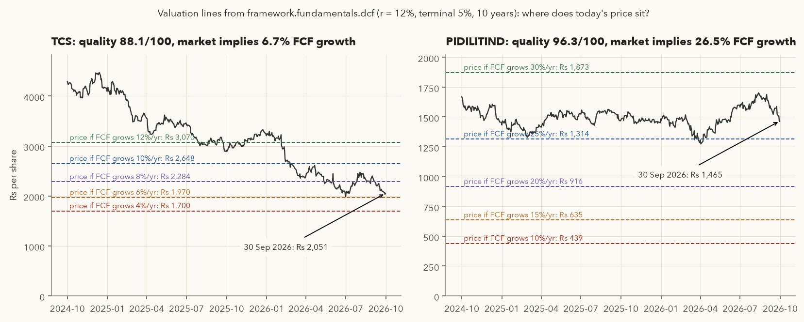
framework.fundamentals.dcf at a different FCF growth rate (r = 12%, terminal 5%, 10 years). The price's position among the lines tells you what growth the market is pricing in."Start buying when the price implies at most two-thirds of historical growth"
- TCS: historical sales CAGR 10.2%, two-thirds is 6.8%. The price lines are Rs 1,970 at 6% and Rs 2,284 at 8%, so the rule's zone starts below roughly Rs 2,100. The 30 Sep close of Rs 2,050.60 sits inside it. Under this rule an investor whose research checklist was also satisfied would buy the first of three tranches, and add the next two only after the next results confirm the thesis or at lower prices.
- Pidilite: historical 14.9%, two-thirds is 9.9%, which corresponds to about Rs 439. Today's Rs 1,465 is more than three times that. The rule says: watchlist only.
- Why tranches: the scorecard is backward-looking and your growth estimate may be wrong. Splitting the buy over 3 dates (or 3 price levels) protects you from buying everything just before bad news. For core holdings this is the same idea as a SIP.
The TCS sensitivity grid runs from Rs 1,742 (r = 13%, g = 6%) to Rs 4,314 (r = 11%, g = 14%). A one-point change in the discount rate moves the value by 15-20%. That is why Varsity insists on a margin of safety (around 30%) and why the framework prints the grid next to the base case.
Sell rules for the core
- Thesis broken: the reason you bought (for example, "pricing power keeps ROCE above 25%") is no longer true for two consecutive years, or the quality score falls below 60.
- Governance: auditor resignation, rising promoter pledging, related-party transactions you cannot explain. Exit first, investigate later.
- Extreme valuation: the reverse DCF implies growth far above anything the business has done (for example, more than 1.5 times its 10-year growth) and the position has grown past your weight cap. Trim back to the cap rather than selling everything.
- Better use of capital: a clearly better business at a clearly better price, after tax. Remember from Chapter 13 that selling within 12 months makes the gain short-term (20% plus cess) instead of long-term (12.5% above the Rs 1.25 lakh yearly exemption).
- Not a sell rule: "the price fell 20%". For the core, a price fall with an intact thesis is a reason to re-check, and possibly to add within your weight cap.
7. Building and sizing the core portfolio
Varsity's Module 9 spends several chapters on portfolio risk: variance, covariance, the correlation matrix, portfolio variance, the equity curve, expected returns and value at risk. The practical lesson for a core portfolio is simple: a portfolio of reasonably uncorrelated stocks swings much less than the stocks in it.
- \(w\)
- The list ("vector") of portfolio weights, one per stock, adding up to 1. Ten equal weights means each is 0.1.
- \(\Sigma\)
- Here capital sigma is not "sum": it is the covariance matrix of daily returns, a table with one row and one column per stock. The diagonal holds each stock's variance (its daily volatility squared); the other cells hold how each pair moves together (their correlation × both volatilities).
- \(w^{\top} \Sigma\, w\)
- (\(\top\) = "transpose", i.e. the weights written as a row.) Shorthand for: for every pair of stocks, multiply weight × weight × their cell in the table, and add everything up. The result is the portfolio's daily variance. It is the two-asset formula from Chapter 11 extended to any number of stocks.
- \(\sqrt{252}\)
- Turns daily volatility into yearly (252 trading days a year).
- \(\sigma_p\)
- The portfolio's annualised volatility, in %.
- 5th percentile
- Sort the past daily portfolio returns from worst to best; the 5th percentile is the return with 5% of days worse than it. It is negative, so the minus sign makes VaR a positive loss.
- \(\text{VaR}_{95\%}\)
- One-day value at risk, in Rs: on 95% of past days the loss was smaller than this.
- Volatility: build the covariance table from the daily returns (a spreadsheet's
COVARIANCE.S, ornumpy.cov), combine it with the weights, take the square root for daily volatility, and multiply by \(\sqrt{252}\). - VaR: this is the historical-simulation method Varsity uses. Compute the portfolio's daily return for every past day, sort them, read off the 5% tail, and multiply by the portfolio value. It says nothing about how bad the worst 5% of days can be; the expected shortfall in the example below covers that.
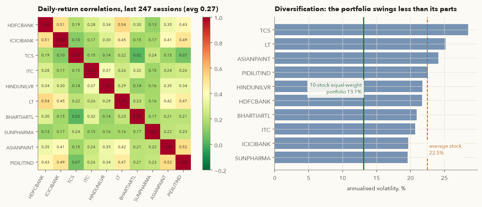
HDFCBANK, ICICIBANK, TCS, ITC, HINDUNILVR, LT, BHARTIARTL, SUNPHARMA, ASIANPAINT, PIDILITIND
- Average annualised volatility of the ten stocks over the last 247 sessions: 22.5%.
- Average pairwise correlation: 0.27 (highest pair HDFCBANK and LT at 0.54; lowest TCS and BHARTIARTL at 0.02).
- Portfolio volatility \(\sqrt{w^\top\Sigma w}\) with \(w_i = 0.1\): 13.1%. Diversification removed about 42% of the swing.
- 1-day 95% historical VaR on Rs 10 lakh: Rs 14,741 (1.47%); the average loss on the worst 5% of days (expected shortfall) was Rs 19,016.
- Portfolio beta to Nifty: 0.90 (beta measures how much the portfolio tends to move for a 1% move in the Nifty; 0.90 means about 0.9%). One-year return -8.9% vs Nifty -8.2%. Diversification lowers volatility; it does not stop a portfolio falling with the market.
Core sizing rules (write your own numbers)
- Number of stocks: 10-20. Below 10, one bad pick hurts too much; above 20, you cannot follow every quarterly result properly.
- Weight caps: at most 10% of the core at cost; trim when a holding passes 15% at market value.
- Sector caps: 25-30% per sector. Banks and financials are a quarter or more of the Nifty, so this cap matters.
- Correlation check: before adding a stock, look at its correlation with what you hold. Two private banks behave more like one position than two.
- Tranches: three buys, spread over time or price, for every new holding.
- Equity curve: track the core's value normalised to 100 against Nifty (Varsity Module 9, "Equity curve"). Underperforming for a year is normal. Underperforming for three years means your selection process needs review.
8. The swing trading framework (satellite bucket)
The swing bucket follows the eight-gate playbook from Chapter 5, now automated by the scanner. The order matters: the market first, then the stock, then the trade.
| Step | Rule in the framework | Why |
|---|---|---|
| 1. Market regime | Score 0-4: Nifty above 200-DMA (+1), 200-DMA rising over 20 days (+1), more than 50% of the universe above its 200-DMA (+1), India VIX below 18 (+1) or above 25 (-1). Score 4 = Risk-on (x1.0 risk), 2-3 = Neutral (x0.5), 1 or less = Risk-off (x0.25) | Breakouts and pullback buys fail more often in falling markets |
| 2. Scanner | RS rating 1-99 (40% 3-month + 60% 6-month relative strength vs Nifty); trend_pullback and breakout_52w setups; watchlist of pullbacks in progress | Leaders keep leading (momentum); trade with the trend |
| 3. Setup check | Open the chart: results date, events, sector exposure, gaps | The code cannot read news or an earnings calendar |
| 4. Size | position_size with regime multiplier, capped at 20% of capital | Same rupee risk on every trade |
| 5. Orders | Buy order for the next session; GTT (good till triggered, a standing broker-side order) stop-loss as soon as it fills | The stop exists even if you are busy at work |
| 6. Management | Trail only upwards, and only after +1R (chandelier: 22-day high minus 3 ATR); exit on the strategy's exit rule | Give winners room, protect open profit |
| 7. Journal | Every entry and exit on the same day | Your real R-multiples, not your memory of them |
| 8. Weekly review | journal stats vs backtest; trailing stops; RS leaders | Catch drift early |
Step 1 in action: the regime over the last two years
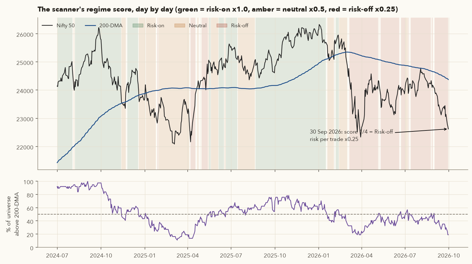
On 30 Sep 2026 the score was 1 out of 4: Nifty at 22,620.45 was 7.2% below its 200-DMA (24,372.85), the 200-DMA was falling, only 19% of the universe was above its own 200-DMA, and only the calm VIX (13.49) earned a point. Two things to notice. First, the label changed 42 times in the 27 months shown, so the multiplier is a dial, not an on/off switch. Second, a low VIX in a falling market is not a reason for comfort; it just means the fall has been orderly.
9. Walking through the 30 Sep 2026 scan
This is the actual output of the scanner on the last day of data, with the default Rs 5 lakh capital and 1% base risk:
$ .venv/bin/python -m framework.scan
=== EOD swing scan for 2026-09-30  |  capital Rs 500,000  |  base risk 1.0% ===

1) MARKET REGIME
   Nifty 22,620.45  (-7.2% vs 200-DMA, -5.4% vs 50-DMA, 200-DMA falling, 1-month -6.1%)
   Breadth: 8% of universe above 50-DMA, 19% above 200-DMA
   India VIX 13.49 (65th percentile of last year)
   => score 1/4: Risk-off. Risk multiplier x0.25 -> effective risk 0.25% per trade

2) RELATIVE STRENGTH LEADERS (vs Nifty; rating 1-99)
              close  ret_3m_pct  ret_6m_pct  from_52w_high_pct  above_50dma  above_200dma  rs_rating
symbol
ADANIENT     2903.4        -8.6        59.3              -10.5        False          True         99
ETERNAL       320.0        14.4        37.2              -13.1         True          True         96
DIXON       13100.0         5.9        30.8              -29.1        False          True         94
HAL          4668.0         5.3        30.1               -9.4        False          True         91
KOTAKBANK     417.0         4.4        13.9               -8.0         True          True         88
TITAN        4587.0         2.4        15.2              -11.6        False          True         86
BAJFINANCE    959.4        -5.8        13.7              -18.4        False         False         83
PIDILITIND   1465.1        -8.7        11.4              -14.2        False         False         80
CDSL         1264.0        -6.4         7.9              -24.5        False         False         78
ICICIBANK    1321.7        -5.6         7.1              -10.7        False         False         75
   ...laggards: HINDUNILVR(14), NTPC(12), ONGC(9), WIPRO(6), INFY(4)

3) SETUPS (signal on close; plan the order for the next session)
   No setups. Doing nothing is a position.

4) WATCHLIST (uptrend + RSI<45: pullback in progress; trigger = close above trigger_above)
   symbol   close  rsi14  vs_50dma_pct  trigger_above  rs_rating
  ETERNAL   320.0  44.48          0.21          329.0         96
    DIXON 13100.0  39.63         -6.32        13425.0         94
      HAL  4668.0  42.70         -3.04         4701.0         91
    TITAN  4587.0  29.49         -7.37         4698.0         86
SUNPHARMA  1816.6  38.95         -4.85         1863.6         57

Checklist before any order: chart looks right? results/events in the next 2 weeks? position <= 20% of capital? total open risk <= 5-6%? Log it: python -m framework.journal add ...
Read it top-down:
- Regime: Risk-off. Base risk 1% becomes 0.25% per trade. In practice, most good swing traders simply take very few trades in such a market.
- RS leaders. ADANIENT (99), ETERNAL (96), DIXON (94), HAL (91) and KOTAKBANK (88) have held up best against the Nifty. Notice that most leaders are below their 50-DMA: even leaders are falling, just less. INFY, WIPRO, ONGC, NTPC and HINDUNILVR are the laggards.
- Setups: none today. "Doing nothing is a position" is a rule, not a slogan.
- Watchlist. Five stocks are in long-term uptrends (above the 200-DMA, 50-DMA above 200-DMA) with RSI below 45. The trigger is a close above today's high (for TITAN, Rs 4,698). These are the names to look at first if the market turns.
After this chapter was written, framework/scan.py was changed to drop any bar where the strategy's exit rule is also true, the same rule run_backtest uses. If you run --days 2 now, the ADANIENT signal below no longer appears. The walkthrough keeps it because it is a good lesson: a scanner hit is only a candidate, and you check it against the system's own rules before you place an order.
Widening the window to two sessions (--days 2) showed this setup from 29 Sep (scanner output before the fix):
$ .venv/bin/python -m framework.scan --days 2        (sections 3 and 5)
3) SETUPS (signal on close; plan the order for the next session)
  symbol          setup signal_date  entry_ref    stop  stop_pct  target_2R  qty  position_value  risk_rs  rs_rating
ADANIENT trend_pullback  2026-09-29     2903.4 2776.65      4.37    3156.91    9         26130.6  1140.79         99
   entry_ref = last close. If tomorrow opens below the stop, skip; if it gaps up >1 ATR, re-size or skip.
5) F&O POSITIONING of setup stocks (near-month futures, latest bhavcopy)
           close  price_chg_pct  oi_chg_pct         buildup  lot_size
symbol
ADANIENT  2902.5           -0.8       -0.28  Long unwinding       309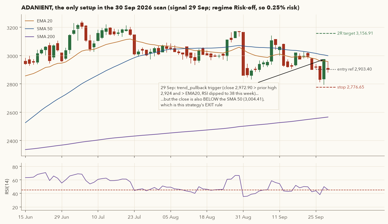
trend_pullback trigger on 29 Sep 2026. Source: NSE data via Yahoo Finance.Checking the setup by hand
- Trend: close 2,972.90 is above the 200-DMA (2,562.17), which is rising; the 50-DMA (3,004.41) is above the 200-DMA. Pass.
- Pullback: RSI(14) fell to 38.1 within the last five sessions (rule: below 45). Pass.
- Trigger: the close of 2,972.90 is above the previous day's high (2,924.00) and above the 20-EMA (2,963.00). Pass.
- Stop: the lower of (5-day low 2,793.70 minus 0.2 x ATR 85.27) = 2,776.65 and (close minus 1 ATR) = 2,887.63, so 2,776.65.
- But: the trigger close of 2,972.90 is below the 50-DMA (3,004.41). The same strategy's exit rule is "close below the 50-DMA". The backtester never buys on a bar where the exit rule is also true; the scanner, as first written, did not apply that filter. So the scanner showed a trade that your backtested system would not have taken.
- Next day: on 30 Sep the stock closed at 2,903.40, down 2.3%, 3.2% below its 50-DMA. The F&O data shows "long unwinding" (futures price -0.8%, open interest -0.28%): longs closing, not fresh buying.
Whatever you trade live must be exactly what you tested. Here the honest response is to skip the trade, and to fix the scanner so it matches the backtest. That fix is now in the framework: scan.find_setups keeps a signal only when entry is true and exit is false, the same rule run_backtest uses. Finding gaps like this between your live process and your tested process is a big part of what the paper-trading stage is for.
Risk-off sizing, then costs
- Risk budget: \(5{,}00{,}000 \times 1\% \times 0.25 = \) Rs 1,250.
- Risk per share: \(2{,}903.40 - 2{,}776.65 = 126.75\). Quantity: \(1{,}250 / 126.75 = 9.86 \Rightarrow\) 9 shares (always round down).
- Actual risk: \(9 \times 126.75 = \) Rs 1,140.75. Position value \(9 \times 2{,}903.40 = \) Rs 26,130.60, only 5.2% of capital. A wide stop makes for a small position.
- Costs from
costs.equity_delivery_charges: if stopped out, charges are Rs 72.29 (STT Rs 51.12, DP charge Rs 15.34, stamp duty Rs 3.92, the rest small), so the net loss is Rs 1,213.04 = -1.06R. If the 2R target of 3,156.91 is hit, charges are Rs 75.84 and the net profit Rs 2,205.75 = +1.93R. - Costs take about 6.3% of the risk amount on a position this small. The Rs 15.34 DP charge is flat per sell, so very small positions are expensive in percentage terms. Chapter 13 covers this in detail.
10. Orders, management and the journal: a full replay
Because 30 Sep 2026 is the end of our data, we cannot see what happens next to ADANIENT. So let us replay a complete trade from a risk-on day, using the scanner's ability to run on a past date:
$ .venv/bin/python -m framework.scan --date 2025-06-30 --days 3        (sections 1 and 3)
=== EOD swing scan for 2025-06-30  |  capital Rs 500,000  |  base risk 1.0% ===

1) MARKET REGIME
   Nifty 25,517.05  (+5.9% vs 200-DMA, +3.1% vs 50-DMA, 200-DMA rising, 1-month +3.1%)
   Breadth: 73% of universe above 50-DMA, 62% above 200-DMA
   India VIX 12.79 (7th percentile of last year)
   => score 4/4: Risk-on. Risk multiplier x1.0 -> effective risk 1.00% per trade
...
3) SETUPS (signal on close; plan the order for the next session)
  symbol        setup signal_date  entry_ref   stop  stop_pct  target_2R  qty  position_value  risk_rs  rs_rating
HDFCBANK breakout_52w  2025-06-26    1000.75 982.46      1.83    1037.33   99        99074.25  1810.88         65
entry_ref = last close. If tomorrow opens below the stop, skip; if it gaps up >1 ATR, re-size or skip.A textbook breakout that failed
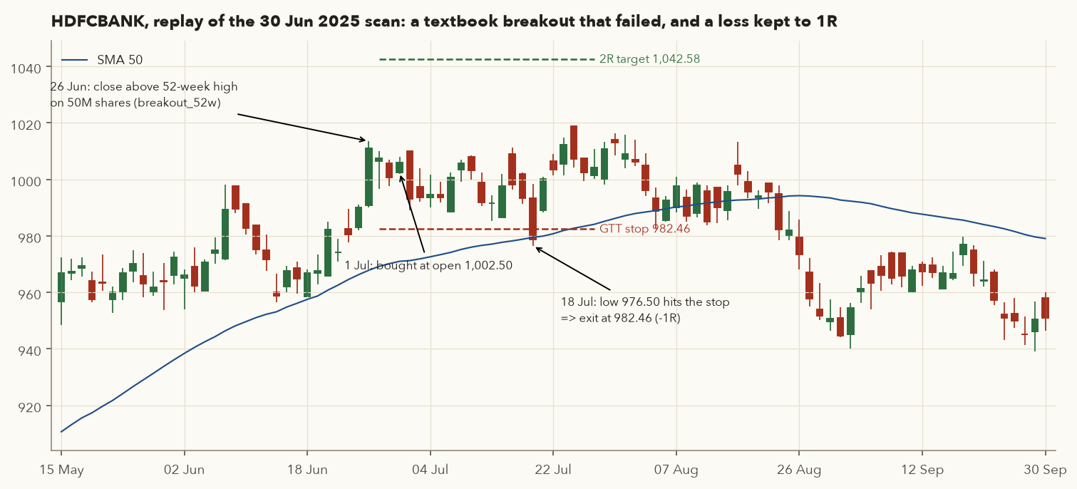
- Regime 4/4, Risk-on: full 1% risk. Signal: on 26 Jun 2025 HDFCBANK closed at a new 52-week high on about 50 million shares, more than 1.5 times its 50-day average volume.
- Size: \(5{,}000 / (1{,}000.75 - 982.46) = 273\) shares by risk, but 273 shares would be Rs 2.7 lakh, above the 20% cap (Rs 1 lakh). The cap wins: 99 shares, risking only Rs 1,811. A tight stop is capped by the position-size limit.
- Orders placed the evening of 30 Jun: a limit buy for 1 Jul, and once it fills, a GTT sell with trigger 982.46. Entry: 1 Jul open at 1,002.50 (risk 20.04 per share; 2R target 1,042.58).
- What happened: the best high before exit was 1,011.35 (only +0.44R). On 18 Jul the low touched 976.50, the GTT triggered, exit at the stop: -1R.
- Was the stop right? By 30 Sep 2025 the stock was at 951.00 after trading as low as 939.10 in Aug-Sep. Following the rule turned a potential -6% into a clean -1R.
GTT orders: the mechanics
- Zerodha's GTT (good till triggered) sits on the broker's server and places a limit order when the trigger price is touched. A single GTT is good for a stop; an OCO (one cancels other) GTT carries both a stop and a target, and cancels one when the other fires. A GTT stays valid for up to one year.
- Because the triggered order is a limit order, set the limit a little below the trigger for a sell stop (for example trigger 982.46, limit 977.55, about 0.5% lower). If the stock gaps below your limit, the order may not fill and you must exit manually. The backtester models this gap risk with its "stop_gap" exits at the open.
- A triggered GTT fires once. If its order does not fill, nothing else protects you; check your orders every evening.
Logging it in the journal
The journal is a CSV file you own (journal/trades.csv). Here is the HDFCBANK trade logged and closed (run with --path scratch.csv so the real journal stays empty; drop --path for your real trades):
$ python -m framework.journal --path scratch.csv add HDFCBANK --entry 1002.5 --stop 982.46 --qty 99 --setup breakout_52w --target 1042.58 --date 2025-07-01 --notes "scan 30-Jun-2025, regime Risk-on"
Added trade #1. Risk = Rs 1,984
$ python -m framework.journal --path scratch.csv close 1 --exit 982.46 --date 2025-07-18 --reason stop
Closed trade #1: net P&L Rs -2,218.05 after Rs 234.09 charges | R = -1.118 net (-1.00 before charges)
Notice the difference between the R before charges (-1.00, the price move from entry to stop) and the net R (-1.118, after Rs 234.09 of charges on two legs of about Rs 1 lakh each). The journal stores the net figure in its r_multiple column, because that is what your account actually lost.
The stats command is the weekly review. Here it is on a demo journal holding the 88 donchian_trend trades entered in 2025-2026 (the "live" sample from Section 4):
$ python -m framework.journal --path demo.csv stats
     closed_trades: 88
       open_trades: 0
          win_rate: 0.227
         avg_win_r: 2.251
        avg_loss_r: 1.037
      expectancy_r: -0.290
     profit_factor: 0.682
         total_pnl: -438365.130
 followed_plan_pct: 100.000
                trades  win_rate  avg_r        pnl
setup
donchian_trend      88     0.227  -0.29 -438365.13
Profit factor 0.68, expectancy -0.29R, win rate 22.7%: on its own a terrible scorecard. Next to the backtest (+0.75R before 2025) it is the clearest possible signal to cut size and investigate. This is the main reason to keep a journal: it is the only honest comparison between the system you tested and the one you are actually running.
The weekly review questions
- Live expectancy, win rate and average win/loss vs the backtest: inside the expected range?
- Rule adherence (
followed_plan_pct): below 90%? Then the problem is you, not the system. - Slippage: were fills worse than planned prices by more than the 0.1% the backtest assumes?
- Open risk: total rupees at risk across open trades still at or below 5-6% of the bucket?
- Trailing stops raised (never lowered) on the weekly chart?
- Sector concentration: three trades in the same sector count as one large bet.
11. The futures framework (last bucket)
Futures (Chapter 9) give leverage, cheap shorting and an efficient hedge. They also turn a normal daily move into a large rupee gain or loss that is settled into your account the same evening. Use them for one of two reasons only, and decide which before you trade.
| Hedging (protect the core) | Directional (swing with leverage) | |
|---|---|---|
| Purpose | Reduce the core's market risk for a few weeks (event risk, a regime turning Risk-off) without selling stocks and paying tax | Express a tested swing signal, long or short |
| When allowed | Any stage, once you understand MTM and margins | Stage 3 only: 6+ months of proven swing results |
| Size | Lots = portfolio value x beta / contract value | Lot-and-stop sizing (below); 0 lots = do not trade |
| Success measure | Portfolio drawdown reduced, at the cost of carry and any upside you give up | Same R-multiple journal as swing trades |
Sizing by lot and stop
The same formula applies, but quantity must be a whole number of lots. position_size(..., lot_size=65, max_position_pct=None) rounds down to whole lots, and it often returns zero.
Can a Rs 10 lakh account trade one Nifty lot at 1% risk?
- Nifty ATR(14) on 30 Sep 2026: 209.0 points. A 2-ATR stop is 418.0 points.
- Risk per lot: \(2 \times 209.0 \times 65 = \) Rs 27,173.
- At 1% risk, capital needed for one lot: \(27{,}173 / 0.01 = \) Rs 27.2 lakh. With a tighter 1-ATR stop, Rs 13.6 lakh.
position_sizereturns 0 lots for Rs 5 lakh, Rs 10 lakh and even Rs 25 lakh. That is the framework telling you the instrument is too big for your account at your risk level.- Stock futures are similar: an ADANIENT lot is 309 shares (about Rs 8.97 lakh of stock); with the scan's stop, one lot risks \(309 \times 126.75 = \) Rs 39,166, almost eight times the 1% budget (Rs 5,000) of a Rs 5 lakh account.
Margin buffer: why "2x margin in cash"
One Nifty lot (65 x 22,707.3 = Rs 14,75,974) needed about Rs 1,67,370 of initial margin on 30 Sep 2026 (SPAN Rs 1,37,851, the exchange's worst-case one-day scenario margin, from NSE's risk file, plus a 2% exposure margin of Rs 29,519): 8.8x leverage. Margin is set to cover a bad day, not a bad month:
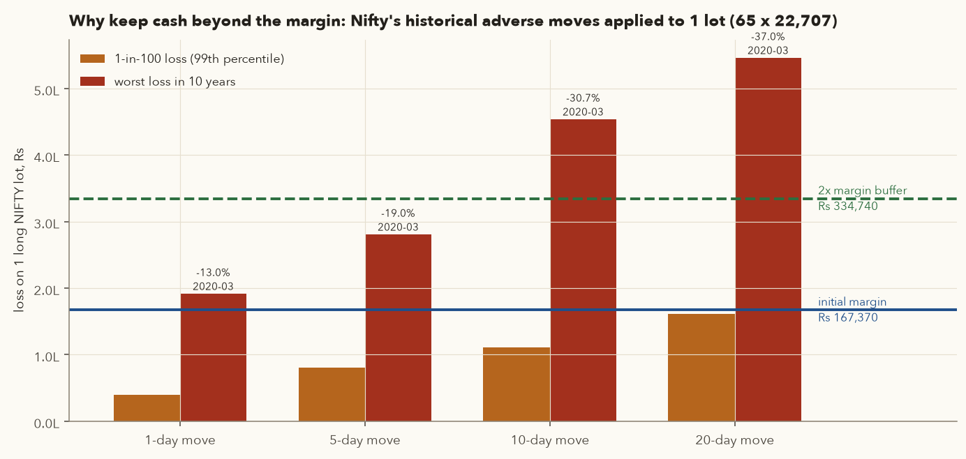
- 1-day: a 1-in-100 day costs about Rs 39,181; the worst day in ten years (23 Mar 2020, -13.0%) about Rs 1,91,588, more than the whole margin.
- 20-day: 1-in-100 about Rs 1,60,920 (-10.9%); the worst, about Rs 5,46,194 (-37.0%).
- Rule: keep at least as much cash again as the margin (2x total) and a hard stop. The stop limits the planned loss; the buffer stops a margin call from forcing you out at the worst moment. Chapter 9's MTM ledger (
futures.mtm_ledger) shows this day by day.
Rollover and OI context
NSE index and stock futures expire on the last Tuesday of the month (the previous trading day if it is a holiday). Positional futures traders roll (close the expiring contract and open the next month's) in the last few days. Open interest (OI) is the number of contracts still outstanding; futures.rollover_pct measures the share of OI already in the next months:
| Date (Sep 2026 series) | 24 Sep | 25 Sep | 28 Sep | 29 Sep (expiry) | Aug expiry day (25 Aug) |
|---|---|---|---|---|---|
| NIFTY rollover % | 40.1 | 50.1 | 63.2 | 74.3 | 77.4 |
| RELIANCE rollover % | 46.4 | 63.4 | 83.7 | 93.7 | 94.7 |
Nifty's September rollover (74.3% on expiry day) was a little lower than August's (77.4%) during a falling month, a mild sign that fewer positions were carried forward. On 30 Sep the OI table showed Short buildup in NIFTY futures (price -0.69%, OI +5.67%) and in HDFCBANK (price -0.91%, OI +0.82%), and Long buildup in BANKNIFTY (price +0.20%, OI +6.09%). Across all F&O symbols: 101 short buildup, 49 long buildup, 36 long unwinding, 28 short covering. Treat this as context that agrees or disagrees with your chart, never as a signal on its own (Chapter 9 explains the four-way OI matrix).
Pricing check: by cost of carry (ignoring dividends due before expiry), fair value for the Oct future with 27 days left is \(22{,}620.45 \times (1 + 0.055 \times 27/365) = 22{,}712.5\); it traded at 22,707.3, a basis of 86.85 points (0.38%), which implies a carry rate of 5.19% a year.
The hedge calculator
- Portfolio value
- The current market value of the holdings you want to protect, in Rs.
- \(\beta\)
- The portfolio's beta to the Nifty: how much it tends to move for a 1% Nifty move (0.90 for the core portfolio in section 7).
- \(F\)
- The price of the Nifty futures contract you short, in index points.
- Lot size
- Units per futures contract (65 for Nifty).
- \(F \times \text{lot size}\)
- The rupee value of one futures lot.
- Lots
- The number of futures lots to sell to offset the portfolio's market risk.
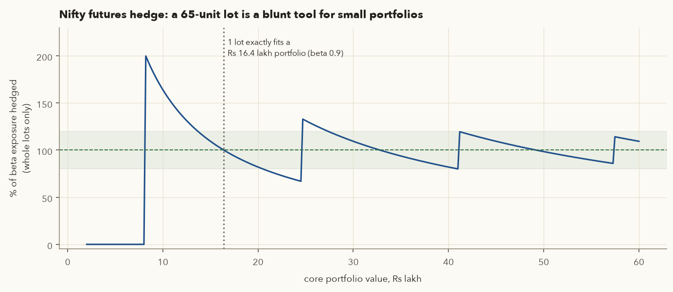
How it works: portfolio value × beta is the "Nifty-equivalent" exposure: how many rupees of Nifty your portfolio behaves like. Divide by one lot's value to see how many lots match it. You can only trade whole lots, so the hedge is usually more or less than 100%; the example below shows how large the rounding error is for small portfolios.
How many lots to short to hedge the core?
- Contract value: \(22{,}707.3 \times 65 = \) Rs 14,75,974.5.
- Rs 10 lakh core: \(10{,}00{,}000 \times 0.90 / 14{,}75{,}974.5 = 0.61\) lots. Rounded to 1 lot = 164% hedged (you would be net short the market).
- Rs 15 lakh: 0.915 lots, 1 lot = 109% hedged. Rs 25 lakh: 1.52 lots, 2 lots = 131%. Rs 50 lakh: 3.05 lots, 3 lots = 98.4%.
- Rs 5 lakh: 0.305 lots rounds to 0. It cannot be hedged with Nifty futures at all.
- No directional futures before Stage 3. No exceptions after a good month.
- If
position_sizereturns 0 lots, the trade is too big. Do not "just do one lot". - At least 2x the initial margin in the account; a stop on every position; never add to a losing futures position.
- Roll in the last 3-4 sessions; never carry a stock future into expiry (physical settlement means you must take or give delivery of the full contract).
- F&O profits are business income taxed at your slab rate, with STT on futures sells at 0.05% from 1 Apr 2026 (Chapter 13).
12. The backtest evidence, read honestly
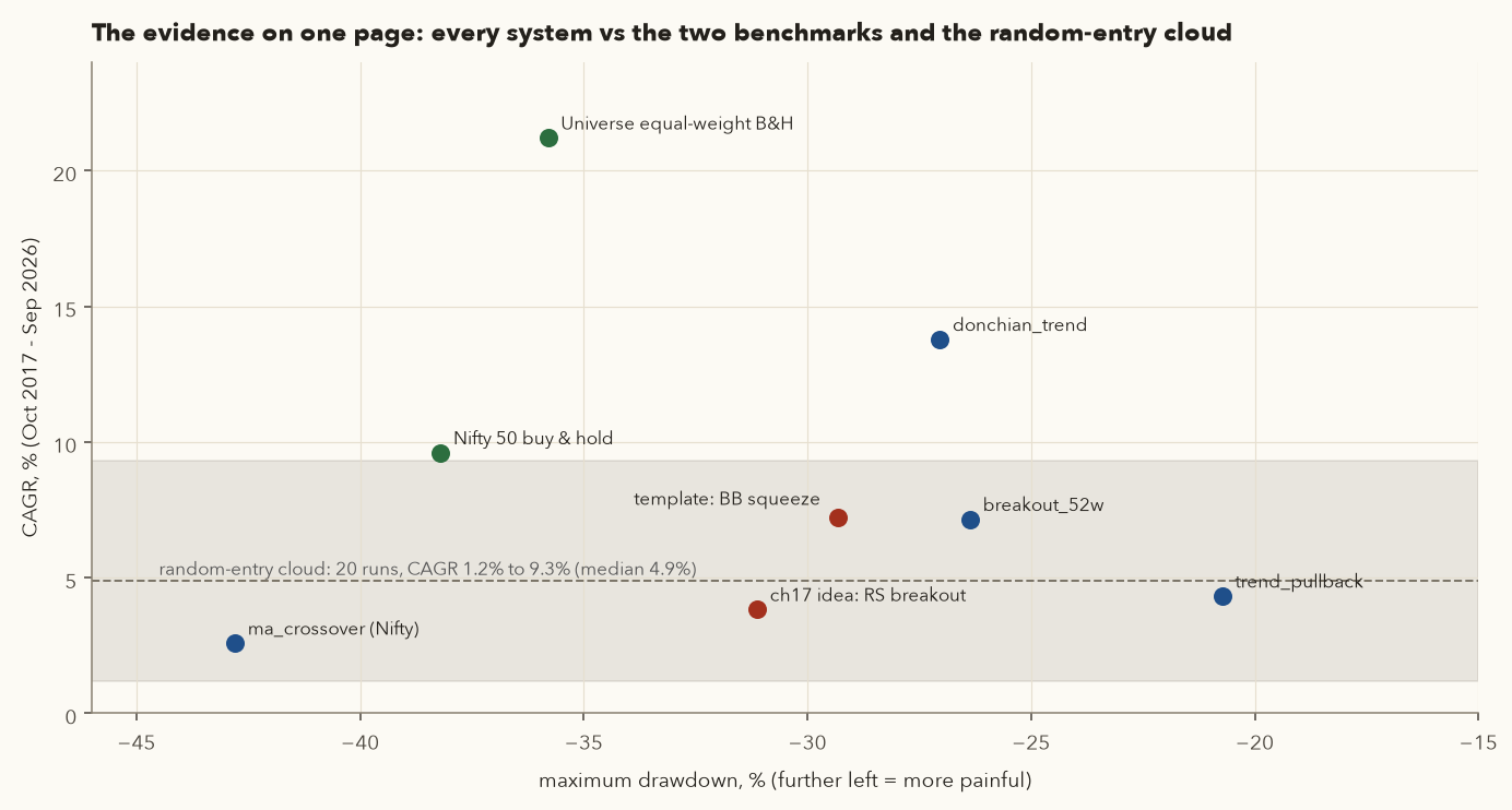
The framework's built-in systems were backtested on the 37-stock universe from Oct 2017 to Sep 2026 with Rs 10 lakh, 1% risk, at most 8 positions and 20% per position, all Indian delivery charges and 0.1% slippage per side (full report in framework/reports/backtest_summary.md; Chapter 12 explains the method).
| System | CAGR | Max DD | Sharpe | Trades | Win % | Exp. (R) | 2017-21 CAGR | 2022-26 CAGR |
|---|---|---|---|---|---|---|---|---|
| trend_pullback | 4.3% | -20.7% | -0.08 | 568 | 29.8% | 0.10 | 8.5% | 0.6% |
| breakout_52w | 7.1% | -26.4% | 0.19 | 388 | 43.3% | 0.12 | 15.5% | 0.2% |
| donchian_trend | 13.8% | -27.0% | 0.58 | 363 | 31.1% | 0.50 | 23.4% | 5.7% |
| ma_crossover (Nifty) | 2.6% | -42.8% | -0.17 | 7 | 42.9% | n/a | 1.9% | 2.9% |
| Nifty 50 buy & hold (price index) | 9.6% | -38.2% | 0.32 | - | - | - | 14.2% | 5.3% |
| Universe equal-weight buy & hold | 21.2% | -35.8% | 0.93 | - | - | - | - | - |
| Random entries, same exits (20 runs) | 1.2% to 9.3% (median 4.9%) | - | - | - | - | - | - | - |
How to read the columns: CAGR is the compound annual growth rate of the equity curve; Max DD is the largest fall from a previous peak; Sharpe is return above the 5.5% T-bill rate divided by volatility (negative means it earned less than T-bills); Exp. (R) is the average trade in R-multiples, net of costs. Chapter 12 derives each one.
What this evidence does and does not say
- Survivorship bias is the biggest issue. The 37 stocks were chosen in 2026 from today's large, successful companies (TRENT, HAL, BEL, DIXON, CDSL, POLYCAB and so on). Simply holding all of them equally returned 21.2% a year, more than twice the Nifty. Nobody could have picked this list in 2017. So the only fair comparison for a stock-picking system on this universe is the equal-weight line, and none of the systems beat it.
- Only
donchian_trendis clearly outside the random cloud (13.8% vs a 9.3% maximum), with a smaller drawdown than buy & hold. Even it made money mostly in 2017-21 (23.4%) and much less in 2022-26 (5.7%), with -19.7% in 2026 to date. - Costs and tax are large. Delivery STT of 0.1% on each side plus slippage cost
trend_pullback4.5 percentage points a year (8.8% before costs, 4.3% after). Swing gains are short-term capital gains, so tax took 22-37% of the systems' P&L. - The parameter sweep is mixed.
donchian_trendworked across entry windows from 20 to 100 days (10.3% to 16.5% CAGR), a sign of robustness.breakout_52wworked only at its default volume filter (1.5x); at 1.0x or 2.0x it dropped to 4.5% and 3.5%, which looks like a fitted parameter. - The honest use of these numbers is to learn how each system behaves: how often it trades, how long it holds, how long its losing streaks are and how deep its drawdowns go. They are not forecasts.
Varsity's momentum portfolio, rebuilt
Module 10's last chapter describes a momentum portfolio: rank a tracking universe by 12-month return, buy the top 10-12 in equal weights, hold for a month, then re-rank and rebalance. Varsity suggests a universe of 150-200 stocks; with only 37 stocks here, treat the result as a demonstration. The figures script rebuilt it with monthly rebalancing and about 0.22% cost per side of turnover:
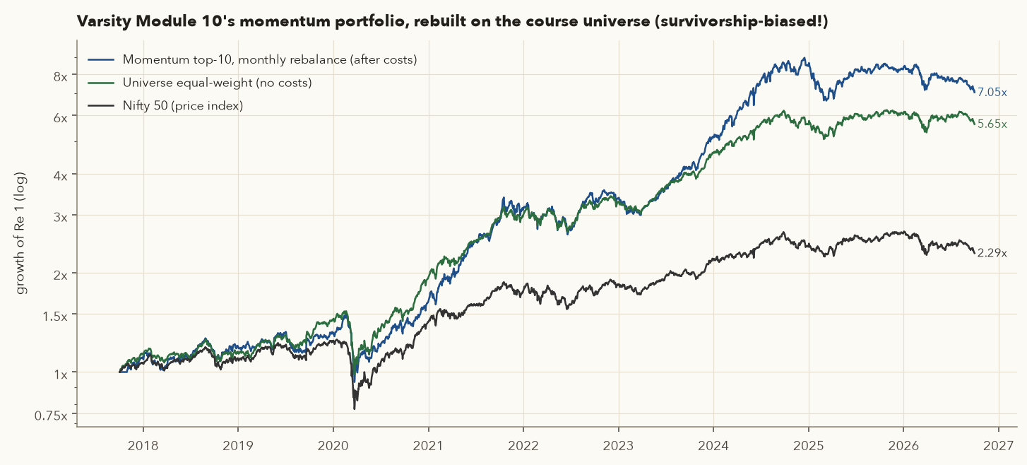
The momentum portfolio beat the equal-weight universe in both halves (30.9% vs 29.5% in 2017-21, a thin margin; 18.4% vs 14.0% in 2022-26), with turnover costs of about 1.0% a year. It is the one idea in this chapter that beat the survivorship-biased benchmark rather than just the Nifty. It still fell 37.5% at its worst, and the universe problem remains, so the next step would be to rerun it on a point-in-time Nifty 100 or Nifty 200 universe before trusting it. Also notice what "momentum" means in a falling market: on 30 Sep 2026 the top-10 list ran from TITAN (+36.7% over 12 months) down to KOTAKBANK (+4.8%), below the T-bill rate. Many momentum investors add an absolute filter (hold cash for a slot if the 12-month return is below the risk-free rate).
Module 10 also covers pair trading (two correlated stocks drift apart and you bet on convergence, using correlation, linear regression, the ADF test and the error ratio) and calendar spreads (trading the price gap between two futures expiries). Both are mean-reversion systems that need F&O, shorting and careful statistics; Chapter 12 introduces them. They belong after Stage 3, not before.
13. Design and test your own strategy, step by step
This is the skill that makes the framework yours. We will do it once, completely, with an idea a learner might reasonably have after reading this course, and we will accept the result even though it is disappointing.
Step 1: write the hypothesis and rules before touching data
"RS leader breakout, only in a healthy market"
- Idea: leaders keep leading (Varsity's momentum logic). A stock beating the Nifty over 6 months that makes a fresh 20-day closing high is showing demand now.
- Regime: Nifty close above its 200-DMA. No new longs otherwise.
- Filter: stock above its 200-DMA; 6-month RS ratio vs Nifty above 1.
- Trigger: close above the highest high of the previous 20 days.
- Stop: close minus 2 x ATR(14). Exit: close below the 50-DMA; chandelier trail armed after +1R.
- Ranking: 6-month RS ratio, strongest first.
- Pass criteria (also written in advance): beat the random-entry cloud's top (9.3%), make money in both 2017-21 and 2022-26, and have neighbouring parameters also work.
Step 2: copy the template and keep the contract
The template (framework/my_strategies/template.py) shows the contract every strategy must honour: return a DataFrame indexed like the input, with entry and exit booleans (decided on the close, filled at the next open), a stop level, an optional trail and target, and a score for ranking. The learner's version (saved for this chapter as course/scripts/ch17_my_idea.py; in your own copy it would live in framework/my_strategies/) is shown below; the file's imports are numpy as np, pandas as pd, framework.indicators as ind and framework.risk.chandelier_stop:
def signals(df: pd.DataFrame, bench: pd.DataFrame | None = None, breakout_n: int = 20, rs_n: int = 126,
            stop_atr: float = 2.0, use_regime: bool = True) -> pd.DataFrame:
    out = df[["open", "high", "low", "close"]].astype(float).copy()
    c = out["close"]

    # --- indicators (all causal: rolling windows and shift(+1) only)
    a = ind.atr(df, 14)
    sma50, sma200 = ind.sma(c, 50), ind.sma(c, 200)
    prior_high = ind.donchian(df, breakout_n)["upper"]            # previous n bars, already shifted
    if bench is not None:
        rs = ind.relative_strength(df, bench, rs_n)["rs_ratio"]
        nb = bench["close"].reindex(c.index).ffill()
        regime = nb > ind.sma(bench["close"], 200).reindex(c.index).ffill()
    else:                                                          # no benchmark: absolute momentum
        rs = (c / c.shift(rs_n)) * 1.0
        regime = pd.Series(True, index=c.index)
    if not use_regime:
        regime = pd.Series(True, index=c.index)

    # --- rules
    leader = (c > sma200) & (rs > 1.0)
    trigger = c > prior_high
    out["entry"] = (regime & leader & trigger).fillna(False).astype(bool)
    out["exit"] = (c < sma50).fillna(False)
    out["stop"] = c - stop_atr * a
    out["trail"] = chandelier_stop(df, 22, 3.0)
    out["target"] = np.nan
    out["score"] = rs
    return out
Every line uses only rolling() windows and donchian(), which is already shifted by one bar. Nothing uses shift(-n) or a whole-series maximum, which would let the strategy see the future.
Step 3: prove it is causal
The framework's test computes the signals on the full history and on history cut off at 31 Mar 2021, and checks they are identical up to that date. If any rule peeks ahead, the two differ:
# run from the repository root with: PYTHONPATH=course/scripts .venv/bin/python check_causal.py
import pandas as pd
from framework.data import load_ohlc
import ch17_my_idea as m
df, b = load_ohlc("RELIANCE"), load_ohlc("NIFTY")
full = m.signals(df, bench=b)
part = m.signals(df.loc[:"2021-03-31"], bench=b.loc[:"2021-03-31"])
cols = ["entry", "exit", "stop", "trail", "score"]
pd.testing.assert_frame_equal(full.loc[part.index, cols], part[cols])   # passes: no look-ahead
In your own copy, add "framework.my_strategies.my_idea:signals" to the parameter list of framework/tests/test_backtest.py::test_strategies_are_causal and run pytest.
Step 4: backtest it with the CLI
$ PYTHONPATH=course/scripts .venv/bin/python -m framework.backtest_cli ch17_my_idea:signals --out my_reports
ch17_my_idea:signals on 37 symbols, 2017-10-03 -> 2026-09-30
              CAGR: 3.8%
               Vol: 12.7%
            Sharpe: -0.07
           Sortino: -0.09
             MaxDD: -31.1%
            Calmar: 0.12
            Trades: 540
          Win rate: 40.7%
     Profit factor: 1.14
    Expectancy (R): 0.04
   Avg hold (days): 30
          Exposure: 83.6%
      Avg invested: 65.1%
        Nifty CAGR: 9.7%
       Nifty MaxDD: -38.4%
Wrote trades/equity/drawdown/metrics to my_reports
--out sends the report files to a folder of your choice; without it they go to framework/reports/ and replace any files with the same name.
Step 5: read the metrics
- CAGR 3.8% is below T-bills (hence the negative Sharpe of -0.07, measured against a 5.5% risk-free rate) and inside the random-entry cloud (median 4.9%).
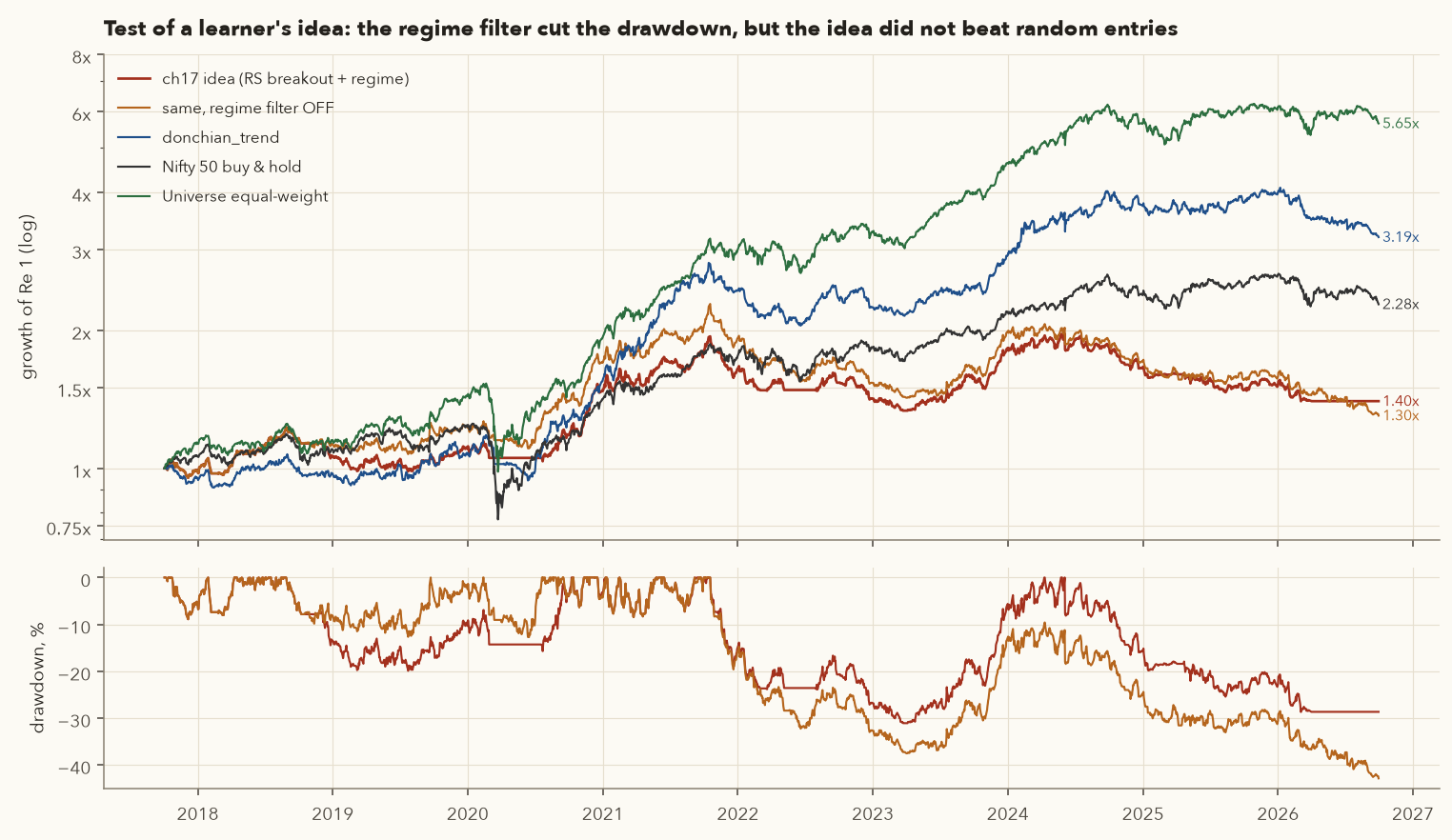
- Profit factor 1.14 but expectancy only 0.04R. Gross rupee wins exceed losses, yet the average trade barely clears zero in R. Wins averaged +1.48R and losses -0.95R with a 40.7% win rate: the exits cut winners early.
- Exit reasons: 430 of 540 trades ended at the stop or trail, 69 on the 50-DMA rule and 41 by gapping through the stop. A 20-day breakout in a trending stock is often the point where short-term buyers are exhausted.
- Costs: Rs 2,40,933 of charges; before costs and slippage the CAGR would have been 6.9%.
Step 6: robustness checks
| Variant (one change at a time) | CAGR | Max DD | Trades | Exp. (R) | PF | 2017-21 | 2022-26 |
|---|---|---|---|---|---|---|---|
| Base (n = 20, 2 ATR, regime on) | 3.8% | -31.1% | 540 | 0.04 | 1.14 | 12.5% | -3.5% |
| Regime filter OFF | 3.0% | -42.9% | 645 | -0.01 | 1.08 | 16.6% | -8.0% |
| Breakout window 10 days | 3.5% | -28.4% | 614 | 0.00 | 1.13 | 7.4% | 0.0% |
| Breakout window 55 days | 2.5% | -36.2% | 493 | 0.00 | 1.10 | 9.9% | -3.9% |
| Stop 3 ATR | 3.9% | -30.9% | 484 | 0.07 | 1.17 | 10.8% | -2.1% |
Step 7: verdict
Rejected, by the criteria written in Step 1. Every variant sits inside the random cloud, and every variant made money in 2017-21 and lost or broke even in 2022-26, which is the market doing the work, not the rule. One useful finding survives: the regime filter cut the maximum drawdown from -42.9% to -31.1% at almost no cost in CAGR. That is worth carrying into other systems (and it is what the scanner's risk multiplier does).
The template's own example (a Bollinger squeeze breakout above the 200-DMA) fares the same way: 7.2% CAGR, -29.3% max drawdown, 595 trades, 0.01R expectancy, and 19.8% in 2017-21 against -3.0% in 2022-26. Most ideas fail. Finding that out for Rs 0 in a backtest, instead of for real money over two years, is the point of the exercise.
The tempting next step is to try 50 more variants until one shows 15% CAGR. With enough tries something always does, by chance. If you test variants, count them, keep the rules you wrote first as the "official" result, and treat the best variant as a new hypothesis to be tested on data it has not seen (another universe, or the next 12 months of paper trading).
Step 8: if it had passed
- Paper-trade it for at least 30 signals with the journal (setup name = your strategy name).
- Register it in
strategies.STRATEGIESand add it toscan.SETUPSso the evening scan shows its signals. The scanner already applies Section 9's rule (no entry on a bar where the exit rule is true), so scan and backtest agree. - Go live at Stage 1 size (0.25%) and compare the journal with the backtest every week.
14. Your written trading plan (fill-in template)
Copy this into a text file, fill in every blank in your own words and numbers, sign and date it. Change it only on the monthly review day, never during market hours or right after a loss.
MY TRADING & INVESTING PLAN                         version ___   date ___________

0. WHY AND HOW MUCH
   Emergency fund (months of expenses) kept outside the market: ____
   Total investable capital: Rs ________   Core ____%   Swing ____%   Futures ____%
   Current stage (0 paper / 1 small / 2 normal / 3 futures): ____

1. CORE (LONG-TERM) RULES
   Universe: ______________________________________________
   Screen: quality score >= ____, Piotroski >= ____, my extra filters: __________
   I must be able to explain the moat and the main risk in two sentences: yes / no
   Buy zone rule: price implies <= ____% of historical growth (reverse DCF), or ________
   Tranches: ____ buys over ____ months.   Max weight per stock ____%   per sector ____%
   Review: after every quarterly result; annual-report read by ________ each year
   Sell rules: thesis broken = ________; governance red flags = ________;
               trim above ____% weight; NOT a reason to sell: ________________

2. SWING RULES
   Systems I trade (tested, with backtest file): ______________________
   Regime filter: ________   Risk per trade: ____% of swing capital x regime multiplier
   Max open risk: ____%   Max positions: ____   Max per position: ____% of swing capital
   Entry order type and time: ________   Skip if gap above entry by > ____ ATR
   Stop: always a GTT, placed ________; I never move a stop down.
   Trail: ________________ (starts after +____R)
   No new trade within ____ days before results / known events.

3. FUTURES RULES (only at stage 3)
   Purpose: hedge / directional.  Max lots: ____.  Cash buffer: >= ____ x margin
   Size: position_size(..., lot_size) must return >= 1 lot at ____% risk
   Roll by ____ sessions before expiry; never hold stock futures into expiry.

4. REVIEW AND DISCIPLINE
   Journal every entry and exit the same day: yes / no
   Weekly: journal stats vs backtest on ________ (day)
   Demotion trigger: live expectancy below backtest's 1st percentile over 50+ trades,
                     or drawdown > ____%, or rule adherence < 90% in a month
   Daily loss stop: if I break a rule, no new trades for ____ sessions.
   Things I know I do wrong (biases): ____________________________

Signed: ______________
15. Routines: daily, weekly, monthly, quarterly
| When | Time | What | Commands |
|---|---|---|---|
| Daily (after 4 pm IST, trading days) | 15-30 min | Refresh data; read the regime line first; review setups on the chart (results dates, events, sector); size; place next-day orders and GTT stops; journal any fills or exits | python -m framework.data updatepython -m framework.scan --capital <swing capital> --risk 1 --save framework/reports/scan_today.txtpython -m framework.journal add/close ... |
| Weekly (weekend) | ~1 hour | Weekly charts of holdings and watchlist; raise trailing stops; RS leaders and laggards, sector rotation; journal stats vs backtest; if trading futures, OI buildup and rollover in expiry week | python -m framework.journal statsfutures.oi_buildup_table(data.load_futures()) |
| Monthly (first weekend) | 1-2 hours | Compare live results with backtest; investigate gaps; update the plan if needed (only now); check open risk and bucket weights; rebalance a momentum sleeve if you run one | python -m framework.backtest_cli all |
| Quarterly (results season) | Half a day | Re-run the scorecard on every core holding and watchlist name after its results; has the quality score, Piotroski or reverse-DCF growth changed? Read results presentation and concall notes; decide on tranches and trims | python -m framework.invest SYMBOL --refresh |
| Yearly (after the 1 Feb Budget and 31 Mar year-end) | Half a day | Update charges and tax rates in config.py and bump AS_OF; review the universe; tax-loss harvesting decisions before 31 Mar; in March, harvest equity LTCG up to the Rs 1.25 lakh exemption and rebalance the core back to its target mix, new money first (Chapters 15-16); read annual reports of core holdings | python -m pytest framework/tests -qpython -m framework.funds harvest --code <scheme> --lots my_lots.csvpython -m framework.funds rebalance --help |
Psychology: the routine protects you from yourself
Varsity's two chapters on trading biases (Module 9) describe the illusion of control (believing that more screen time or more indicators gives you control over outcomes), recency bias (over-weighting the last few events or trades), anchoring (fixating on your buy price or an old high), functional fixedness (using a tool only the way you first learned it), confirmation bias (seeking only evidence that agrees with you) and attribution bias (crediting wins to skill and blaming losses on the market). Varsity's suggested cure for the last one is a trading journal. Each routine above defends against one of them: fixed rules against the illusion of control, weekly statistics over many trades against recency, a valuation range written in advance against anchoring, the backtest-vs-journal comparison against attribution, and the written plan against all of them. Chapter 11 adds loss aversion, overconfidence and revenge trading, and covers each in depth.
16. The 12-week learning roadmap
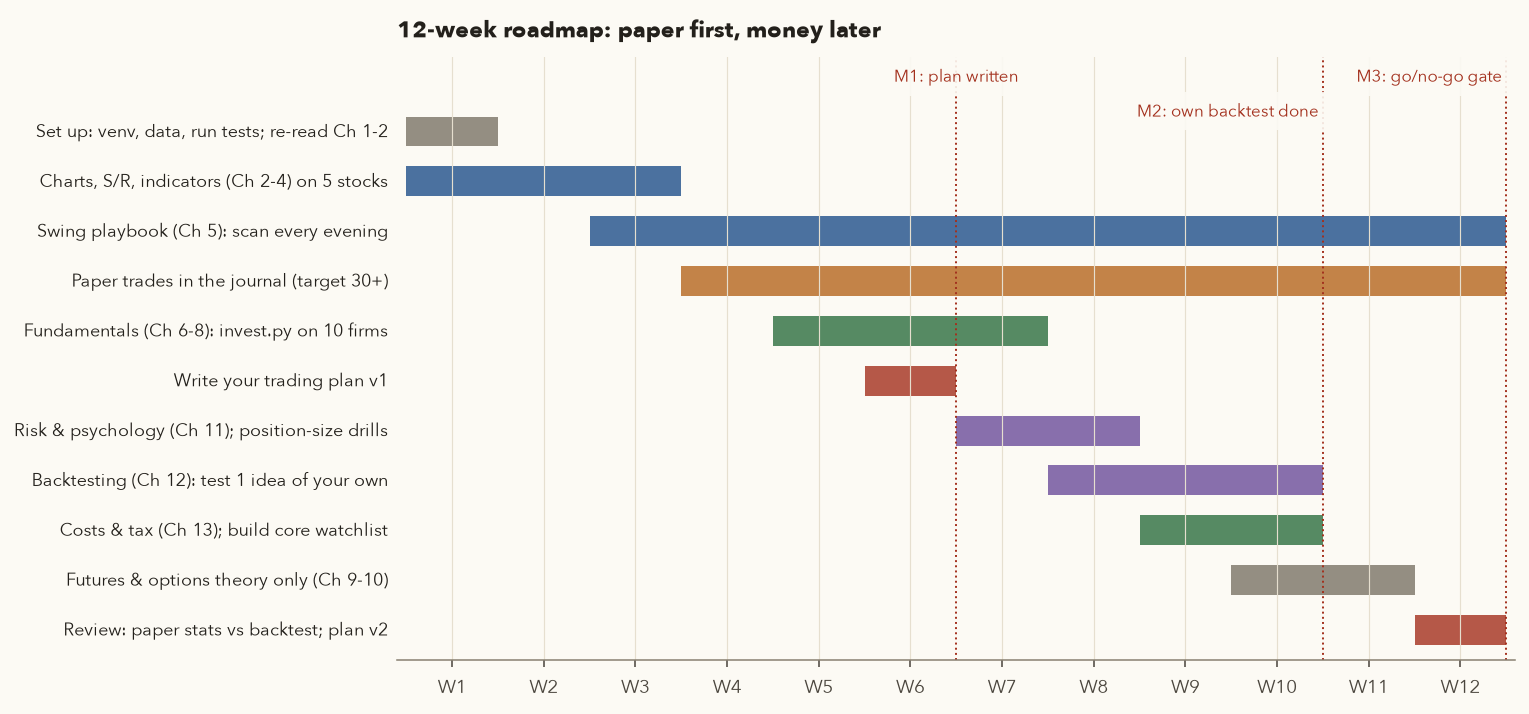
| Weeks | Focus | Milestone you can check |
|---|---|---|
| 1 | Install, run tests, load data; reread Chapters 1-2 | pytest passes; you can plot any stock's weekly chart |
| 1-3 | Charts, support/resistance, indicators on 5 stocks you know | For each stock: trend, key levels, ATR, RSI written down |
| 3-12 | Evening scan every trading day | A dated folder of saved scan files |
| 4-12 | Paper trades in the journal, at the size the plan would use | 30+ paper trades, every one with a stop and a setup name |
| 5-7 | Fundamentals: invest.py on 10 companies; read 2 annual reports | A one-page note per company: moat, risks, buy zone |
| 6 | Write trading plan v1 (Section 14) | M1: signed plan |
| 7-8 | Risk and psychology; sizing drills until automatic | Size 20 hypothetical trades by hand, then check with position_size |
| 8-10 | Backtest one idea of your own (Section 13) | M2: written verdict with robustness table |
| 9-10 | Costs and tax; build the core watchlist | Net-of-cost P&L for your paper trades; 10-name watchlist with buy zones |
| 10-11 | Futures and options theory only | Compute margin, MTM and a hedge for your own numbers |
| 12 | Review paper stats against the backtest; plan v2 | M3: go/no-go. Go to Stage 1 only if the Stage 0 exit criteria are all met |
The core bucket can start earlier than the swing bucket. Staggered buying of a few high-quality businesses in tranches, or an index fund while you learn (Chapter 14), does not need a proven trading edge. It needs the research checklist and patience.
17. Keeping data fresh and extending the framework
Daily prices
# after ~4 pm IST (Yahoo is sometimes a day late)
.venv/bin/python -m framework.data update                 # every CSV in data/ohlc
.venv/bin/python -m framework.data update TCS NIFTY       # just these
update_ohlc re-downloads the last ten days from Yahoo Finance and overwrites them, so provisional bars get corrected. Two cautions. First, vendors sometimes miss corporate actions: the framework found three by scanning for overnight gaps above 20% (the Tata Motors demerger in Oct 2025, a TRENT adjustment and a CDSL listing-day bar) and back-adjusts them through config.PRICE_ADJUSTMENTS. Run that gap check after every update of a new symbol. Second, never mix adjusted and unadjusted prices in the same calculation: charts use split-adjusted closes, while backtests use dividend-adjusted (adjust=True) total-return prices. A third, smaller one: an incremental update does not rewrite older Adj Close values when a new dividend goes ex, so the adjusted series slowly drifts from Yahoo's. Once or twice a year, move a CSV aside and run update for that symbol to re-download its full 10-year history.
F&O bhavcopy
NSE publishes a daily F&O bhavcopy (UDiFF format) at a URL of the form https://nsearchives.nseindia.com/content/fo/BhavCopy_NSE_FO_0_0_0_YYYYMMDD_F_0000.csv.zip. Download it with a browser User-Agent, keep the futures rows and append them to data/fno/. data.load_futures() reads the file named in config.FUTURES_FILE, so point that setting at your updated file. Lot sizes change periodically; always take them from the latest bhavcopy rather than from memory.
Fundamentals
fetch_fundamentals caches each company in data/fundamentals/SYMBOL.json for 7 days; use --refresh after results. It tries the consolidated page first and falls back to standalone. Screener's "+" breakdown rows are not fetched, so items like receivables days and NPA ratios come from the company's own filings.
Rates and rules
Every charge and tax rate lives only in framework/config.py, with a source comment and an AS_OF date (currently 2 Oct 2026). As of that date it encodes: delivery STT 0.1% on buy and sell, futures STT 0.05% on sell (from 1 Apr 2026), options STT 0.15% of premium on sell, stamp duty 0.015% on delivery buys, a Rs 15.34 DP charge per sell, STCG 20% and LTCG 12.5% above Rs 1.25 lakh a year, plus 4% cess. The fund rules used by framework.funds (the three tax classes and their holding periods, 0.005% stamp duty on fund purchases, 0.001% STT on equity-fund and equity-ETF sales) sit in the same file under the MF_ names. After every Budget or SEBI circular, check the broker's charges page and the brokerage calculator, update config.py, bump AS_OF and rerun the tests.
Extension points
- Universe: edit
config.UNIVERSE, thenpython -m framework.data update NEWSYM. A point-in-time universe (for example, Nifty 100 constituents as of each year) is the single biggest improvement you can make to backtest honesty. - Strategies:
framework/my_strategies/, following Section 13. - Scorecard: the rule list in
fundamentals.quality_scorecard; each rule is(name, value, weight, zero_at, full_at). Add your own (for example receivable days) and keep the weights visible. - Scanner: add your strategy to
scan.SETUPS. The entry-and-not-exit filter from Section 9 is already built in. - Tests: every new function deserves a test; every new strategy goes into the causality test.
18. Try it yourself
These snippets need a copy of the course repository (set up as in its framework/README.md). Save each as a .py file and run it from the repository's root folder, for example .venv/bin/python snippet.py. Outputs shown are from the course data to 30 Sep 2026.
A. Size and cost a planned swing trade
import sys; sys.path.insert(0, ".")          # run from the repository root
from framework import risk, costs

capital, base_risk, regime_mult = 500_000, 1.0, 0.25      # Risk-off on 30 Sep 2026
entry, stop = 2903.40, 2776.65                            # ADANIENT plan from the scan
qty = risk.position_size(capital, base_risk * regime_mult, entry, stop, max_position_pct=20)
target = 3156.91                                          # 2R target printed by the scan
print("qty", qty, "| risk Rs", round(qty * (entry - stop), 2), "| target", round(target, 2))
for label, exit_px in [("stop", stop), ("target", target)]:
    c = costs.equity_delivery_charges(entry, exit_px, qty)
    print(label, "charges", c["total"], "net P&L", c["net_pnl"])
qty 9 | risk Rs 1140.75 | target 3156.91
stop charges 72.29 net P&L -1213.04
target charges 75.84 net P&L 2205.75B. Screen companies on quality and implied growth
import sys; sys.path.insert(0, ".")          # run from the repository root
from framework import fundamentals as F

for sym in ["TCS", "PIDILITIND", "ITC"]:
    fin = F.fetch_fundamentals(sym)                 # uses the 7-day cache in data/fundamentals/
    sc = F.quality_scorecard(sym, fin)
    v = F.valuation_snapshot(fin)                   # r = 12%, terminal 5%, 10 years
    print(f"{sym:<11} quality {sc['score']:5.1f} ({sc['grade']})  P/E {v['pe']:5.1f}  "
          f"implied FCF growth {v['implied_growth']:.1%}  vs 5y sales CAGR {v['growth_assumed']:.1%}")
TCS quality 88.1 (A) P/E 14.0 implied FCF growth 6.7% vs 5y sales CAGR 10.2%
PIDILITIND quality 96.3 (A) P/E 56.1 implied FCF growth 26.5% vs 5y sales CAGR 14.9%
ITC quality 83.3 (A) P/E 16.2 implied FCF growth 9.7% vs 5y sales CAGR 9.9%C. How sure are you about a system's edge?
import sys; sys.path.insert(0, ".")          # run from the repository root
import numpy as np, pandas as pd
from framework.risk import expectancy

t = pd.read_csv("framework/reports/donchian_trend_trades.csv")
r = t["r_multiple"].dropna()
e = expectancy(r)
se = r.std() / np.sqrt(len(r))
print(f"n={e['n']}  E={e['expectancy']:.2f}R  win={e['win_rate']:.1%}  payoff={e['payoff']:.2f}")
print(f"standard error {se:.3f}R -> 90% interval {e['expectancy']-1.645*se:.2f}R to {e['expectancy']+1.645*se:.2f}R")
print("trades needed for E>0 at 95% confidence:", int(np.ceil((1.645 * r.std() / r.mean()) ** 2)))
n=363 E=0.50R win=31.1% payoff=3.78
standard error 0.189R -> 90% interval 0.19R to 0.81R
trades needed for E>0 at 95% confidence: 142D. Core portfolio beta and the hedge
import sys; sys.path.insert(0, ".")          # run from the repository root
import pandas as pd
from framework import data, futures as fu

core = ["HDFCBANK", "ICICIBANK", "TCS", "ITC", "HINDUNILVR", "LT", "BHARTIARTL", "SUNPHARMA", "ASIANPAINT", "PIDILITIND"]
nifty = data.load_ohlc("NIFTY")["close"]
betas = pd.Series({s: fu.beta(data.load_ohlc(s, adjust=True)["close"], nifty, 250) for s in core})
port_beta = betas.mean()                                   # equal weights
print(betas.round(2).to_string()); print("portfolio beta", round(port_beta, 2))
print(fu.beta_hedge(1_500_000, round(port_beta, 2), fut_price=22707.3, lot=65))
HDFCBANK 1.25
ICICIBANK 0.93
TCS 0.80
ITC 0.65
HINDUNILVR 0.76
LT 1.43
BHARTIARTL 0.63
SUNPHARMA 0.48
ASIANPAINT 1.01
PIDILITIND 1.09
portfolio beta 0.9
{'hedge_value': 1350000.0, 'contract_value': 1475974.5, 'lots_exact': 0.9146499482206502, 'lots': 1, 'hedged_pct': 109.33144444444444}Exercise: replace the trades CSV in snippet C with your own journal (journal/trades.csv, column r_multiple) once you have 30 closed paper trades.
19. Framework checklist
- Emergency fund and insurance are in place outside the market.
- Capital is split into core, swing and futures buckets, with written percentages and a current stage.
- Every core holding passed the screen, has a written thesis (moat plus main risk) and was bought in tranches inside a pre-decided buy zone.
- No core stock is above the weight cap; no sector above the sector cap.
- If the core holds funds: one fund per asset class, a written target allocation, and a March harvest-and-rebalance check.
- Every swing strategy I trade has a backtest that beats the random-entry cloud, works in both halves of history and has a causality test.
- The scanner and the backtest use exactly the same rules (including "no entry when the exit rule is true").
- Every open trade has a GTT stop in place; total open risk is within the limit.
- Every trade is in the journal, with setup name, stop, costs, R and whether I followed the plan.
- Weekly: live statistics compared with the backtest's range; demotion rule checked.
- Futures only at Stage 3, sized by lot and stop, with at least 2x margin in cash.
config.pyrates checked after the latest Budget/SEBI change; tests pass.- The written plan is signed, dated and changed only on review days.
20. Key takeaways
- A trading system is a written, repeatable process: inputs, fixed logic, an output and a decision rule. If you cannot write it down, you cannot test it or follow it.
- Use three buckets with separate rules: a fundamental core (most of the money), a technical swing satellite, and futures only after a proven swing edge.
- Edges are measured with large error. About 140 trades were needed to show that a +0.50R trend system was probably real; 30 trades mainly test your discipline.
- For the core: screen on quality, read the reports, value with a range, buy in tranches inside a buy zone, review every quarter, and sell when the thesis breaks, not when the price dips.
- For swing trades: regime first, then scanner, chart check, fixed-risk sizing, a GTT stop, trailing only upwards, and a journal entry the same day.
- On 30 Sep 2026 the framework said Risk-off and showed no setups. Looking back one more session found one candidate, which on inspection your tested system would not have taken (the scanner now filters such cases out). Skipping trades is part of the system.
- Futures: a Nifty lot with a 2-ATR stop needs about Rs 27 lakh of capital at 1% risk; keep 2x margin in cash; small portfolios hedge poorly with a 65-unit lot.
- Backtests here are survivorship-biased; the fair benchmark is the equal-weight universe (21.2%). Only
donchian_trendand the momentum portfolio cleared the random-entry cloud, and both did much worse after 2021. - Most new ideas fail, like the RS-breakout idea in Section 13. Test, accept the verdict, keep what is useful (here, the regime filter) and move on.
- Keep data, rates and the plan current. Paper first, money later.
21. Quiz and exercises
Q1. Your swing bucket is Rs 3 lakh, the regime is Neutral, base risk is 1%. Entry 1,250, stop 1,190. How many shares, and what is the rupee risk?
Q2. A paper-trading record shows 30 trades with expectancy +0.6R and an R standard deviation of 2.5. Is the edge proven?
Q3. On 30 Sep 2026, run with --days 2, the original scanner listed ADANIENT as a trend_pullback setup from 29 Sep. Give two reasons from this chapter to skip it.
Q4. The reverse DCF for a company says the price implies 22% FCF growth for 10 years. Its 10-year sales CAGR is 12%. What does your framework say to do?
Q5. Why does the framework use a different valuation for HDFC Bank than for TCS? Compute the justified P/B for ROE 17%, g = 5%, r = 12%.
Q6. A Rs 20 lakh core portfolio has beta 1.1. NIFTY futures trade at 22,707.3 with a lot of 65. How many lots hedge it, and what percentage is hedged?
Q7. Your backtest shows 18 consecutive losses at worst. What drawdown does that imply at 0.5%, 1% and 3% risk per trade?
Q8. A new strategy returns 8.5% CAGR on the course universe vs 9.6% for Nifty buy & hold and 21.2% for the equal-weight universe. The random-entry cloud is 1.2% to 9.3%. What do you conclude?
Q9. Your live journal after 60 trades shows expectancy -0.4R. The backtest's bootstrap for 60 trades has a 1st percentile of -0.15R. What does your plan say?
followed_plan_pct), regime (is the market in a phase the backtest rarely saw?) and whether the scanner matches the tested rules.Q10. In Section 13 the regime filter did not raise CAGR much (3.0% to 3.8%). Why might you still keep it?
Q11. Exercise: run python -m framework.scan --date 2025-06-30 --days 3 and --date 2026-09-30. What changed in the regime inputs?
Q12. Exercise: list three ways the framework's backtests could overstate real results, and the fix for each.
22. Sources
Zerodha Varsity, Module 10 "Trading Systems": module page, ch. 1 What is a trading system? (What to expect), ch. 2 Pair trading logic, ch. 15 Calendar spreads, ch. 16 Momentum portfolios.
Zerodha Varsity, Module 9 "Risk Management & Trading Psychology": module page, Risk (Part 1), Risk (Part 2) variance and covariance, Risk (Part 4) correlation matrix and portfolio variance, Equity curve, Expected returns, Position sizing for active traders, Part 2, Part 3, Kelly's criterion, Trading biases, Trading biases (Part 2).
Zerodha Varsity, Module 3 "Fundamental Analysis": Investment due diligence (the checklist), Equity research (Part 1), Equity research (Part 2): DCF and intrinsic value.
Framework code and reports (in the course repository): framework/README.md, framework/reports/backtest_summary.md (backtests to 30 Sep 2026), framework/config.py (charges and tax rates with sources, AS_OF 2 Oct 2026).
Data: daily OHLCV for NSE stocks and indices via Yahoo Finance (to 30 Sep 2026); NSE F&O UDiFF bhavcopy Aug-Sep 2026 (NSE); NSE SPAN risk parameters for 30 Sep 2026 (via Chapter 9's data file); fundamentals from screener.in TCS, PIDILITIND, HDFCBANK, ITC (fetched Oct 2026).
Rules and rates: Zerodha charges and brokerage calculator; ClearTax, STT rates after Budget 2026; ICICI Direct, STT changes in Budget 2026; Zerodha support, GTT validity; Zerodha Z-Connect, Introducing GTT; Business Standard on SEBI's FY25 F&O study (July 2025).
Figures and numbers: course/scripts/ch17_figures.py (writes data/extra/ch17_numbers.json) and course/scripts/ch17_my_idea.py.